Wave Equation: double slit domain

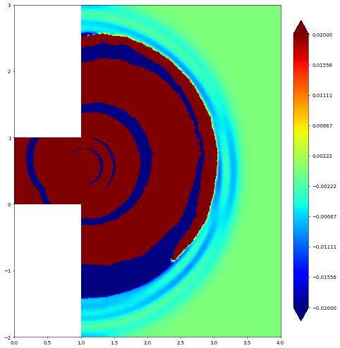
In the following we will consider the wave equation \begin{align*} \partial_{tt}\psi - \Delta\psi &= 0, && \text{in } \Omega\times(0,T), \\ \psi &= g, && \text{on } \Gamma_D\times(0,T), \\ \nabla\psi\cdot n &= 0 && \text{on } \partial\Omega\setminus\Gamma_D, \end{align*} where \(n\) is the outward unit normal and \(g\) is given Dirichlet data given on part of the domain boundary. We repeat a double slit experiment, i.e., we have a wave channel which ends in two slits on the right and forcing the wave on the left end by defining \(g=\frac{1}{10\pi}\cos(10\pi t)\).

We discretize the wave equation by an explicit symplectic time stepping scheme for two unknowns \(\psi^n\) and \(p^n\) where \(p=-\partial_t\psi\) based on \begin{align*} \partial_t \psi = -p, \\ \partial_t p = -\triangle\psi \end{align*} The discretization first updates \(\psi\) by half a time step then updates \(p\) and concludes by another update step for \(\psi\). So given \((\psi^n,p^n)\) we compute \begin{align*} \psi^{n+\frac{1}{2}} &= \psi^n - \frac{\Delta t}{2}p^n, \\ p^{n+1} &= \begin{cases} p^n - \triangle\psi^{n+\frac{1}{2}} & \text{in the interior}, \\ g(t^{n+1}) & \text{on }\Gamma_D \end{cases} \\ \psi^{n+1} &= \psi^{n+\frac{1}{2}} - \frac{\Delta t}{2}p^{n+1}. \end{align*} Note that the update for \(\psi\) does not involve any spatial derivatives so can be performed directly on the level of the degree of freedom vectors. We use numpy for these steps. For the update of \(p\) we use a variational formulation \begin{align*} \vec{p} &= \vec{p} + M^{-1}S\vec{\psi} \end{align*} where \(S\) is the stiffness matrix \(S=(\int_\Omega\nabla\varphi_j\nabla\varphi_i)_{ij}\) and \(M\) is the mass matrix, i.e., \(M=\int_\Omega\varphi_j\varphi_i)_{ij}\). To simplify the computation we use a lumped version of this matrix, i.e,, \(M\approx{\rm diag}(\int_\Omega\varphi_i)\). In this form the algorithm only involves a matrix vector multiplication and no implicit solving step is required.

The following test case is taken from https://firedrakeproject.org/demos/linear_wave_equation.py.html

from matplotlib import pyplot as plt
import numpy
import dune.fem as fem
from dune.grid import reader
from dune.alugrid import aluConformGrid as leafGridView
from dune.fem.space import lagrange as solutionSpace
from ufl import TrialFunction, TestFunction, grad, dot, dx
from dune.ufl import Constant, BoxDirichletBC
T = 3
dt = 0.005
t = 0

We use gmsh to define the domain and then set up a first order scalar Lagrange space which we will use both for \(\psi\) and \(p\). We can construct general grids by either defining the grids directly in Python (as demonstrated in the following example) or by reading the grid from files using readers provided by Dune, e.g., Dune Grid Format (dgf) files or Gmsh files.

domain = (reader.gmsh, "wave_tank.msh")
gridView  = leafGridView( domain, dimgrid=2 )
gridView.hierarchicalGrid.loadBalance()
V = solutionSpace(gridView, order=1, storage="numpy")

p      = V.interpolate(0,name="p")
phi    = V.interpolate(0,name="phi")
pVec   = p.as_numpy
phiVec = phi.as_numpy

Next we define an operator for the stiffness matrix including the boundary condition which are time dependent so we use a Constant for this. We use the BoxDirichletBC class which is derived from the more general DirichletBC class which takes a function space, the boundary function \(g\) as a ufl expression, and finally a description of the part \(\Gamma_D\) of the boundary where this boundary condition is defined. This can be a ufl expression which evaluates to \(0\) for \(x\not\in\Gamma_D\), e.g., an ufl conditional.

Note that the stiffness matrix does not depend on time so we can assemble the matrix once and extract the corresponding scipy sparse matrix.

u    = TrialFunction(V)
v    = TestFunction(V)
p_in = Constant(0.0, name="g")
# the following is equivalent to
# x    = SpatialCoordinate(V)
# bc   = DirichletBC(V, p_in, conditional(x[0]<1e-10,1,0))
bc   = BoxDirichletBC(V, p_in, [None,None],[0,None], eps=1e-10)

from dune.fem.operator import galerkin
op        = galerkin([dot(grad(u),grad(v))*dx,bc])
S         = op.linear().as_numpy
lapPhi    = V.interpolate(1,name="e")
lapPhiVec = lapPhi.as_numpy

Next we construct a lumped (diagonal) approximation \(M\) to the mass matrix. We then use this to form the matrix \(\Delta t M^{-1}S\) where \(M^{-1}\) is easy to compute since \(M\) is diagonal. To compute \(M\) we can either use the row sum approach which is a diagonal matrix with entries \(m_{ii} = \sum_j\int_\Omega\varphi_i\varphi_j\). We could either setup a mass matrix using

M = galerkin(u*v*dx).linear().as_numpy
diag = M.sum(axis=1)

Another approach is to construct a mass operator \(<L[u],\varphi_i> = \int_\Omega u\varphi_i\) and applying that to \(u\equiv 1\):

from scipy.sparse import dia_matrix
lumping = galerkin(u*v*dx)
lumped = lapPhi.copy()
lumping(lapPhi,lumped)       # note that lapPhi=1
N = len(lumped.as_numpy)
M = dia_matrix(([dt/lumped.as_numpy],[0]),shape=(N,N) )
S1 = M*S

An alternative approach is to use an interpolation quadrature, where the integral for the mass matrix \int_:nbsphinx-math:Omega `:nbsphinx-math:varphi`_i:nbsphinx-math:varphi_j$ is approximated by a quadrature based on the Lagrange points. We can change the quadrature by using the metadata argument when defining the ufl measure:

Todo

currently mass lumping only for schemes

from dune.fem.scheme import galerkin
lumping = galerkin(u*v*dx(metadata={"quadrature_rule":"lumped"})==0)
lumped = lumping.linear().as_numpy.diagonal()
M = dia_matrix(([dt/lumped],[0]),shape=(N,N) )
S2 = M*S

We can now set up the time loop and perform our explicit time stepping algorithm. Note that the computation is carried out completely using numpy and scipy algorithms we the exception of setting the boundary conditions. This is done using the setConstraints method on the stiffness operator which we constructed passing in the boundary conditions. At the time of writing it is not yet possible to extract a sparse matrix and vector encoding the boundary constraint.

step = 0
while t <= T:
    step += 1
    phiVec[:] -= pVec[:]*dt/2
    pVec[:]   += S2*phiVec[:]
    t += dt
    # set the values on the Dirichlet boundary
    p_in.value = numpy.sin(2*numpy.pi*5*t)
    op.setConstraints(p)
    phiVec[:] -= pVec[:]*dt/2
phi.plot(gridLines=None, clim=[-0.02,0.02], figure=plt.figure(figsize=(10,10)))

This page was generated from the notebook wave_nb.ipynb and is part of the tutorial for the dune-fem python bindings