Tweaking the (non-) linear solvers
Here we look at how to tweak the internal linear and nonlinear solvers. The solve method on the schemes uses a Newton method to solve the (non)linear PDE model. Parameters set during the construction of a scheme can be used to customize the Newton solver and the underlying solver for the linear problem in each step, i.e., setting line-search parameters or preconditioners. A number of linear solvers and some simple preconditioners are directly available and others can be used through
additional software packages. This is done by changing the linear algebra backend (e.g. using petsc) by using the storage parameter during construction of the discrete space. The simplicity of the default backend (numpy) allows to extract the underlying data structures to use with Numpy/Scipy on the python side. A degrees of freedom vector (dof vector) can be retrieved as numpy.array from a discrete function with this default storage by using the as_numpy attribute on an
instance of a discrete function. Similar attributes are available for the other storages, i.e., as_istl,as_petsc. The same attributes are also available to retrieve the underlying matrix structures on linear operators/schemes. A short description on the other storages with examples using the internal bindings for these packages follows at the end of this section. We will discuss how to use these attributes to implement (parts of) the solution algorithm on the Python side using Scipy or
PETSc4py will follow.
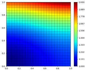
We will mostly revisit the nonlinear problem studied at the end of the section on non-linear elliptic problems in the introduction - using a prescribed forcing to obtain the exact solution \begin{align*} u(x,y) = \left(\frac{1}{2}(x^2 + y^2) - \frac{1}{3}(x^3 - y^3)\right) + 1 \end{align*} The following code was described in the introduction
[1]:
import numpy

from dune.grid import structuredGrid as leafGridView
from dune.fem.space import lagrange
from dune.fem import integrate
from ufl import TestFunction, TrialFunction, SpatialCoordinate, FacetNormal, \
                dx, ds, div, grad, dot, inner, exp, sin, conditional

gridView = leafGridView([0, 0], [1, 1], [24, 24])
space = lagrange(gridView, order=2)
u_h = space.interpolate(0, name='u_h')

x,u,v,n = ( SpatialCoordinate(space), TrialFunction(space), TestFunction(space), FacetNormal(space) )
exact = 1/2*(x[0]**2+x[1]**2) - 1/3*(x[0]**3 - x[1]**3) + 1

a  = ( inner(grad(u),grad(v)) + (1+u)**2*u*v ) * dx
bf = (-div(grad(exact)) + (1+exact)**2*exact) * v * dx
bg = dot(grad(exact),n)*v*ds

# simple function to show the result of a simulation
def printResult(method,error,info):
    print(method,"L^2, H^1 error:",'{:0.5e}, {:0.5e}'.format(
                 *[ numpy.sqrt(e) for e in integrate([error**2,inner(grad(error),grad(error))]) ]),
          "\n\t","solver info=",info,flush=True)
When creating a scheme, it is possible to set the linear solver as well as parameters for the internal Newton solver and the linear solver (e.g. for preconditioning). See a list of available solvers and preconditioning methods at the end of this section. The default solver is a gmres method but since this problem is symmetric a cg solver is more efficient. In addition we will use a Jacobi preconditioner and set the tolerance for the Newton method
to \(10^{-8}\):
[2]:
from dune.fem.scheme import galerkin
scheme = galerkin(a == bf+bg, solver='cg',
                  parameters={"linear.preconditioning.method":"jacobi",
                              "nonlinear.tolerance":1e-7},
                 )
Tip
we use Krylov methods like cg and gmres in this section to solve the linear problems. We also provide bindings for direct solvers from the suitesparse package, e.g., umfpack if installed. For this use solver=["suitesparse","umfpack"] when constructing the scheme.
We can simply use the galerkin scheme instance to compute the solution as shown previously in the introduction section.
[3]:
u_h.interpolate(2)               # start with the boundary conditions at the top
info = scheme.solve(target=u_h)
printResult("Default",u_h-exact,info)
u_h.plot()
Default L^2, H^1 error: 1.17596e-06, 1.83002e-04
         solver info= {'converged': True, 'iterations': 4, 'linear_iterations': 459, 'timing': [0.093334123, 0.017711429, 0.075622694]}
Python sided Newton solver
We can also only use the internal linear solvers and write the Newton method in Python - here is a very simple version of that. The central new method is linear available on the scheme that returns a linear scheme which represents the Jacobian of the model around a given grid function ubar. Much more details on the methods used are given in the next section.
[4]:
class Scheme1:
    def __init__(self, scheme, u0):
        self.scheme = scheme
        self.jacobian = scheme.linear(ubar=u0) # obtain a linear operator for the Newton method

    def solve(self, target):
        # create a copy of target for the residual
        res = target.copy(name="residual")
        dh  = target.copy(name="direction")
        n, linIter = 0,0
        while True:
            # res = S[u]
            #     = u - g on boundary
            self.scheme(target, res)
            absF = res.scalarProductDofs(res)
            if absF < 1e-7**2: # this is the same tolerance we set above for the built-in Newton solver
                break
            self.scheme.jacobian(target,self.jacobian)  # assemble the linearization
            # dh = DS[u]^{-1}S[u]
            #    = u - g on boundary
            dh.clear()
            info = self.jacobian.solve(target=dh,rightHandSide=res)
            linIter += info["linear_iterations"]
            # unew = u - DS[u]^{-1}S[u]
            #      = u - (u-g) = g on boundary
            target -= dh
            n += 1
        return {"iterations":n, "linear_iterations":linIter}

u_h.interpolate(2)                        # start with the boundary conditions at the top
scheme_cls = Scheme1(scheme,u0=u_h)
info = scheme_cls.solve(target=u_h)
printResult("Newton 1",u_h-exact,info)
Newton 1 L^2, H^1 error: 1.17596e-06, 1.83002e-04
         solver info= {'iterations': 4, 'linear_iterations': 459}
Tip
The iterative linear solvers use the provided target discrete function as initial guess for the iteration - so here we are starting with 0 in each step of the Newton method.
A second version using a linearization of the non-linear problem including an affine shift, i.e., the first two terms in the Taylor expansion around a given \(\bar{u}\):
[5]:
from dune.fem.scheme import linearized
class Scheme2:
    def __init__(self, scheme, u0):
        self.scheme = scheme
        # let's use a `gmres` solver for demonstration purposes
        self.linear = linearized(scheme, ubar=u0,
                      parameters={ "method":"gmres", "gmres.restart":50 })

    def solve(self, target):
        prev = target.copy()
        n, linIter = 0,0
        # we are not computing the residual directly so need a different
        # stopping criteria, i.e., size of the step dh
        while True:
            # setup L[u] = DS[u^n](u-u^n) + S[u^n]
            # Then L[u] = 0 leads to
            # u = (DS[u^n])^{-1} (DS[u^n]u^n-S[u^n])
            #   = u^n - DS[u^n])^{-1}S[u^n]
            #   = u^{n+1}
            self.linear.setup(target)
            info = self.linear.solve(target=target)
            linIter += info["linear_iterations"]

            # We don't have access to the residual so we use |u^{n+1}-u^n|
            # as stopping criteria.
            # Subtract the new iterate from the previous one
            prev.sub( target )
            absDiff = prev.scalarProductDofs(prev)
            if absDiff < 1e-7**2:
                break
            prev.assign(target)
            n += 1
        return {"iterations":n, "linear_iterations":linIter}

u_h.clear()                         # reset u_h - so we start the Newton method with u_h=0
scheme_cls = Scheme2(scheme,u_h)
info = scheme_cls.solve(target=u_h)
printResult("Newton 2 (gmres)",u_h-exact,info)
Newton 2 (gmres) L^2, H^1 error: 1.17601e-06, 1.83002e-04
         solver info= {'iterations': 8, 'linear_iterations': 2076}
Tip
the parameters used to tweak the linear solver set when constructing the scheme are passed on to the linear solver when calling scheme.linear but can be overwritten. Below we construct a linearization (by default around zero) which uses a gmres method when calling jac.solve - the same would work with sc.linear(parameter={..}).
Here is another example of this:
[6]:
model = ( inner(grad(u), grad(v)) + (u - conditional(dot(x,x)<0.6,10.,0.))*v ) * dx
# verbose output for the linear solver is too long so use default `False` setting
sc  = galerkin(model==0, solver="cg",
               parameters={"linear.verbose":False,"nonlinear.verbose":True}
              )
sol = space.interpolate(0, name="u_h")
jac = linearized(sc, parameters={ "method":"gmres", "gmres.restart":100, })
info = jac.solve(target=sol)
print(info,flush=True)
{'converged': True, 'iterations': 0, 'linear_iterations': 1106, 'timing': []}
Since we setup the scheme using solver="cg" calling the solve method will use the Newton method with a cg solver - some verbose output is provided in each step of the Newton method due to "nonlinear.verbose":True:
[7]:
sol.clear()
info = sc.solve(target=sol)
print(info,flush=True)
{'converged': True, 'iterations': 0, 'linear_iterations': 213, 'timing': [0.027243577, 0.004660004, 0.022583573000000003]}
Tip
since the problem is linear the Newton method produces no real overhead.
Handling Dirichlet boundary conditions
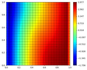
We first look at a simple Poisson problem with Dirichlet BCs to show how to use the internal solvers in this setting. We solve \(-\triangle u=15\chi_\omega\) where \(\chi_\omega\) is a characteristic function with \(\omega=\{x\colon |x|^2<0.6\}\). For the boundary we prescribe trivial Neumann at the top and bottom boundaries and Dirichlet values \(u=-1\) and \(u=1\) at the left and right boundaries, respectively.
[8]:
from dune.ufl import DirichletBC
model = ( inner(grad(u), grad(v)) - 15*conditional(dot(x,x)<0.6,1.,0.) * v ) * dx
dbcs  = [ DirichletBC(space,-1,1), DirichletBC(space, 1,2) ]
op  = galerkin([model==0, *dbcs], space)
sol = space.interpolate(0, name="u_h")
lin = op.linear()
So far everything is as before. Dirichlet boundary conditions are handled in the matrix through changing all rows associated with boundary degrees of freedom to unit rows - associated columns are not changed so the matrix will not be symmetric anymore. For solving the system we need to modify the right hand side and the initial guess for the iterative solver to include the boundary values (to counter the missing symmetry). We can use the first of the three versions of the setConstraints
methods on the scheme class discussed in the section on more general boundary conditions.
[9]:
op.setConstraints(sol)

# setup the right hand side
rhs = sol.copy()
op(sol,rhs)
rhs *= -1
op.setConstraints(rhs)
lin.solve(rightHandSide=rhs,target=sol)
sol.plot()
Let’s revisit our two implementations of the Newton method discussed above but with Dirichlet conditions on the whole boundary:
[10]:
scheme = galerkin([a == bf, DirichletBC(space,exact)], solver='cg')
First version with scheme.linear:
[11]:
u_h.interpolate(2)                        # start with the boundary conditions at the top
scheme_cls = Scheme1(scheme,u0=u_h)
info = scheme_cls.solve(target=u_h)
printResult("Dirichlet, Newton 1",u_h-exact,info)
Dirichlet, Newton 1 L^2, H^1 error: 1.17658e-06, 1.83002e-04
         solver info= {'iterations': 4, 'linear_iterations': 414}
and using the linearized operator:
[12]:
u_h.interpolate(2)
scheme_cls = Scheme2(scheme,u0=u_h)
info = scheme_cls.solve(target=u_h)
printResult("Dirichlet, Newton 2",u_h-exact,info)
Dirichlet, Newton 2 L^2, H^1 error: 1.17659e-06, 1.83002e-04
         solver info= {'iterations': 4, 'linear_iterations': 518}
Other internal solvers (petsc)
The following requires that a PETSc installation was found during the configuration of dune.
[13]:
from dune.common.checkconfiguration import assertCMakeHave, ConfigurationError
try:
    assertCMakeHave("HAVE_PETSC")
    petsc = True
except ConfigurationError:
    print("Dune not configured with petsc - skipping example")
    petsc = False
We provide internal bindings to parts of the PETSc package and show this first. How to make use of petsc4py is shown in a later section.
Switching to a storage based on the PETSc solver package and solving the system using the dune-fem bindings can be achieved by using the storage argument to the space constructor.
Note
We can use the ufl forms we already have defined. Normally the space to use is extracted from the form but this can be overwritten by providing a space argument during scheme construction.
We’ll use Dirichlet BCs at the left boundary only:
[14]:
if petsc:
    spacePetsc = lagrange(gridView, order=2, storage='petsc')
    # We use an sor preconditioner:
    schemePetsc = galerkin([a == bf+bg, DirichletBC(space,exact,2)],
                           space=spacePetsc, solver="cg",
                           parameters={"linear.preconditioning.method":"hypre"})
    uPetsc_h = spacePetsc.interpolate(2, name='u_h')
    info = schemePetsc.solve(target=uPetsc_h)
    printResult("PETSc",uPetsc_h-exact,info)
PETSc L^2, H^1 error: 1.17613e-06, 1.83002e-04
         solver info= {'converged': True, 'iterations': 4, 'linear_iterations': 22, 'timing': [0.092794927, 0.057642113, 0.035152814]}
Other internal solvers (istl)
We can just as easily use the dune-istl package to solve the system (dune-istl should be available when installing dune-fem).
Tip
instead of changing the storage in the space requiring some extra compilation it is also possible to provide the solver information directly to the scheme as shown here.
[15]:
spaceIstl = lagrange(gridView, order=2, storage='istl')
# We use an amg preconditioner:
schemeIstl = galerkin(a == bf+bg, solver=("istl","cg"),
                      parameters={"linear.preconditioning.method":"amg-jacobi"})
u_h.interpolate(2)
info = schemeIstl.solve(target=u_h)
printResult("Dune-Istl",u_h-exact,info)
Dune-Istl L^2, H^1 error: 1.17597e-06, 1.83002e-04
         solver info= {'converged': True, 'iterations': 4, 'linear_iterations': 42, 'timing': [0.184266485, 0.035994204, 0.148272281]}
Parameters for fine-tuning the internal solvers
Sometimes it is necessary to extract which parameters were read and which values were used, e.g., for debugging purposes like finding spelling in the parameters provided to a scheme. Note that this information can only be reliably obtained after usage of the scheme, e.g., after calling solve as shown in the example below. To add logging to a set of parameters passed to a scheme one simply needs to add a logging key to the parameter dictionary provided to the scheme with a tag (string)
that is used in the output.
As an example we will solve the simple Laplace equation from the introduction but pass some preconditioning parameters to the scheme.
[16]:
import dune.fem
from dune.grid import structuredGrid
from dune.fem.space import lagrange
from ufl import (TestFunction, TrialFunction, SpatialCoordinate,
                 dx, grad, inner, dot, sin, cos, pi )
gridView = structuredGrid([0, 0], [1, 1], [200, 200])
space = lagrange(gridView, order=1)
u_h   = space.interpolate(0, name='u_h')
x = SpatialCoordinate(space)
u = TrialFunction(space)
v = TestFunction(space)

f = (8*pi**2+1) * cos(2*pi*x[0])*cos(2*pi*x[1])
a = ( inner(grad(u),grad(v)) + u*v ) * dx
l = f*v * dx
scheme = galerkin( a==l, solver="cg", parameters=
                   {"linear.tolerance": 1e-12,
                    "linear.verbose": True,
                    "linear.preconditioning.method": "jacobi",
                    "linear.errormeasure": "relative",
                    "logging": "log-jacobi"
                   } )
info = scheme.solve(target=u_h)
Fem::CG preconditioning=jacobi
Fem::CG it: 0 : sqr(residuum) 9.91003e-26
Fem::CG it: 1 : sqr(residuum) 1.1676e-26
We use the pprint (pretty print) module if available to get nicer output.
[17]:
try:
    from pprint import pprint as _pprint
    pprint = lambda *args,**kwargs: _pprint(*args,**kwargs,width=200,compact=False)
except ImportError:
    pprint = print

pprint(dune.fem.parameter.log())
{'default': {('fem.dofmanager.clearresizedarrays', 'true'), ('fem.dofmanager.memoryfactor', '1.1'), ('fem.threads.communicationthread', 'false'), ('fem.solver.threading', 'true')},
 'log-jacobi': {('fem.solver.linear.maxiterations', '2147483647'),
                ('fem.solver.linear.preconditioning.iterations', '1'),
                ('fem.solver.linear.preconditioning.relaxation', '1.1'),
                ('fem.solver.linear.threading', 'true'),
                ('fem.solver.nonlinear.forcenonlinear', 'false'),
                ('fem.solver.nonlinear.forcing', 'none'),
                ('fem.solver.nonlinear.linesearch', 'none'),
                ('fem.solver.nonlinear.maxiterations', '2147483647'),
                ('fem.solver.nonlinear.maxlinesearchiterations', '2147483647'),
                ('fem.solver.nonlinear.simplified', 'false'),
                ('fem.solver.nonlinear.tolerance', '1e-06'),
                ('fem.solver.nonlinear.verbose', 'false'),
                ('linear.errormeasure', 'relative'),
                ('linear.method', 'cg'),
                ('linear.preconditioning.method', 'jacobi'),
                ('linear.tolerance', '1e-12'),
                ('linear.verbose', 'True')},
 'program code': {('fem.adaptation.method', 'callback')}}
Note above that all parameters are printed including some default ones used in other parts of the code. If multiple schemes with different logging parameter strings are used, all would be shown using the log method as shown above. To access only the parameters used in the scheme simply use either dune.fem.parameter.log()["tag"]) or access the parameter log through the scheme:
[18]:
pprint(scheme.parameterLog())
{('fem.solver.linear.maxiterations', '2147483647'),
 ('fem.solver.linear.preconditioning.iterations', '1'),
 ('fem.solver.linear.preconditioning.relaxation', '1.1'),
 ('fem.solver.linear.threading', 'true'),
 ('fem.solver.nonlinear.forcenonlinear', 'false'),
 ('fem.solver.nonlinear.forcing', 'none'),
 ('fem.solver.nonlinear.linesearch', 'none'),
 ('fem.solver.nonlinear.maxiterations', '2147483647'),
 ('fem.solver.nonlinear.maxlinesearchiterations', '2147483647'),
 ('fem.solver.nonlinear.simplified', 'false'),
 ('fem.solver.nonlinear.tolerance', '1e-06'),
 ('fem.solver.nonlinear.verbose', 'false'),
 ('linear.errormeasure', 'relative'),
 ('linear.method', 'cg'),
 ('linear.preconditioning.method', 'jacobi'),
 ('linear.tolerance', '1e-12'),
 ('linear.verbose', 'True')}
One can easily reuse these parameters to construct another scheme by converting the result of the above call to a dictionary. As an example change the above problem to a PDE with Dirichlet conditions but turn off verbose output of the solver.
Note
The logging parameter has to be set if we want to use the parameterLog method on the scheme.
[19]:
param = dict(scheme.parameterLog()) # this method returns a set of pairs which we can convert to a dictionary
param["logging"] = "Dirichlet" # only needed to use the `parameterLog` method
param["linear.verbose"] = False
scheme2 = galerkin( [a==l,DirichletBC(space,0)], parameters=param )
u_h.interpolate(2)
info = scheme2.solve(target=u_h)
pprint(scheme2.parameterLog())
{('fem.solver.linear.maxiterations', '2147483647'),
 ('fem.solver.linear.preconditioning.iterations', '1'),
 ('fem.solver.linear.preconditioning.relaxation', '1.1'),
 ('fem.solver.linear.threading', 'true'),
 ('fem.solver.nonlinear.forcenonlinear', 'false'),
 ('fem.solver.nonlinear.forcing', 'none'),
 ('fem.solver.nonlinear.linesearch', 'none'),
 ('fem.solver.nonlinear.maxiterations', '2147483647'),
 ('fem.solver.nonlinear.maxlinesearchiterations', '2147483647'),
 ('fem.solver.nonlinear.simplified', 'false'),
 ('fem.solver.nonlinear.tolerance', '1e-06'),
 ('fem.solver.nonlinear.verbose', 'false'),
 ('linear.errormeasure', 'relative'),
 ('linear.method', 'cg'),
 ('linear.preconditioning.method', 'jacobi'),
 ('linear.tolerance', '1e-12'),
 ('linear.verbose', 'False')}
Tip
To get information about available values for some parameters (those with string arguments) a possible approach is to provide a non valid string, e.g., "help".
[20]:
try:
    scheme = galerkin( a==l, solver="cg", parameters=
                       {"linear.tolerance": 1e-12,
                        "linear.verbose": True,
                        "linear.preconditioning.method": "help",
                        "linear.errormeasure": "relative",
                        "logging": "precon"
                       } )
    scheme.solve(target=u_h)
except RuntimeError as rte:
    print(rte)
Help for parameter 'fem.solver.linear.preconditioning.method':
Valid values are: none, sor, ssor, gauss-seidel, jacobi
Available solvers and parameters
Upon creation of a discrete function space one also have to specifies the storage which is tied to the solver backend. As mentioned, different linear algebra backends can be accessed by changing setting the storage parameter during construction of the discrete space. All discrete functions and operators/schemes based on this space will then use this backend. Available backends are numpy,istl,petsc. Note that not all methods which are available in dune-istl or PETSc have been
forwarded to be used with dune-fem.
[21]:
space = lagrange(gridView, order=2)
Switching is as simple as passing storage='istl' or storage='petsc'. Here is a summary of the available backends
Solver |
Description |
|---|---|
numpy |
the storage is based on a raw C pointer which can be |
directly accessed as a numpy.array using the Python buffer protocol |
|
To change the underlying vector of a discrete function |
|
|
|
As shown in the examples, linear operators return a |
|
|
|
istl |
data is stored in a block vector/matrix from the dune.istl package |
Access through |
|
petsc |
data is stored in a petsc vector/matrix which can also be used with |
petsc4py on the python side using |
When creating a scheme, there is the possibility to select a linear solver for the internal Newton method. In addition the behavior of the solver can be customized through a parameter dictionary. This allows to set tolerances, verbosity, but also which preconditioner to use.
For details see the help available for a scheme:
[22]:
help(scheme)
Help on Scheme in module dune.generated.femscheme_1830e0b499d58f20cb34ce353560f035 object:

class Scheme(pybind11_builtins.pybind11_object)
 |  A scheme finds a solution `u=ufl.TrialFunction` for a given variational equation.
 |  The main method is `solve` which takes a discrete functions as `target` argument to
 |  store the solution. The method always uses a Newton method to solve the problem.
 |  The linear solver used in each iteration of the Newton method can be chosen
 |  using the `solver` parameter in the constructor of the scheme. Available solvers are:
 |  ------------------------------------------
 |  |  Solver  |         Storage             |
 |  |   name   |  numpy  |  istl   |  petsc  |
 |  |----------|---------|---------|---------|
 |  | bicg     |   ---   |   ---   |    x    |
 |  | bicgstab |    x    |    x    |    x    |
 |  | cg       |    x    |    x    |    x    |
 |  | gmres    |    x    |    x    |    x    |
 |  | gradient |   ---   |    x    |   ---   |
 |  | loop     |   ---   |    x    |   ---   |
 |  | minres   |   ---   |    x    |    x    |
 |  | preonly  |   ---   |   ---   |    x    |
 |  | superlu  |   ---   |    x    |   ---   |
 |  ------------------------------------------
 |
 |  In addition the direct solvers from the `suitesparse` package can be used with the
 |  `numpy` storage. In this case provide a tuple as `solver` argument with "suitesparse" as
 |  first argument and the solver to use as second, e.g.,
 |  'solver=("suitesparse","umfpack")'.
 |
 |  The detailed behavior of the schemes can be customized by providing a
 |  `parameters` dictionary to the scheme constructor, e.g.,
 |     {"nonlinear.tolerance": 1e-3,       # tolerance for newton solver
 |      "nonlinear.verbose": False,        # toggle iteration output
 |      "nonlinear.maxiterations": maxInt, # max number of nonlinear iterations
 |      "nonlinear.linesearch": True,      # use a simple bisection line search
 |      "nonlinear.forcing": "none",       # can switch to eisenstatwalker
 |      "nonlinear.simplified": False,     # use a quasi Newton method with single Jacobian evaluation
 |
 |      "linear.tolerance": 1e-5,          # tolerance for linear solver
 |      "linear.verbose": False,           # toggle linear iteration output
 |      "linear.maxiterations":1000,       # max number of linear iterations
 |      "linear.errormeasure": "absolute", # or "relative" or "residualreduction"
 |
 |      "linear.preconditioning.method": "jacobi",          # (see table below)
 |      "linear.preconditioning.hypre.method": "boomeramg", #  "pilu-t" "parasails"
 |      "linear.preconditioning.iteration": 3,              # iterations for preconditioner
 |      "linear.preconditioning.relaxation": 1.0,           # omega for SOR and ILU
 |      "linear.preconditioning.level": 0}                  # fill-in level for ILU preconditioning
 |  -----------------------------------------------
 |  |  Precondition | (x = parallel | s = serial) |
 |  |  method       |  numpy  |   istl  |  petsc  |
 |  |---------------|---------|---------|---------|
 |  | amg-ilu       |   ---   |    x    |   ---   |
 |  | amg-jacobi    |   ---   |    x    |   ---   |
 |  | gauss-seidel  |    x    |    x    |    x    |
 |  | hypre         |   ---   |   ---   |    x    |
 |  | icc           |   ---   |   ---   |    x    |
 |  | ildl          |   ---   |    x    |   ---   |
 |  | ilu           |   ---   |    s    |    s    |
 |  | jacobi        |    x    |    x    |    x    |
 |  | kspoptions    |   ---   |   ---   |    x    |
 |  | lu            |   ---   |   ---   |    s    |
 |  | ml            |   ---   |   ---   |    x    |
 |  | none          |    x    |    x    |    x    |
 |  | oas           |   ---   |   ---   |    x    |
 |  | pcgamg        |   ---   |   ---   |    x    |
 |  | sor           |    x    |    x    |    x    |
 |  | ssor          |    x    |    x    |    x    |
 |  -----------------------------------------------
 |
 |  The functionality of some of the preconditioners listed for petsc will
 |  depend on the petsc installation.
 |
 |  Method resolution order:
 |      Scheme
 |      pybind11_builtins.pybind11_object
 |      builtins.object
 |
 |  Methods defined here:
 |
 |  __call__(...)
 |
 |  __init__(...)
 |
 |  dirichletIndices = _opDirichletIndices(self, id=None)
 |
 |  inverseLinearOperator(...)
 |
 |  jacobian(...)
 |
 |  linear = _linearized(scheme, ubar=None, assemble=True, parameters={}, onlyLinear=True)
 |
 |  setErrorMeasure(...)
 |
 |  setQuadratureOrders(...)
 |
 |  solve(scheme, target, rhs=None, *, rightHandSide=None)
 |
 |  ----------------------------------------------------------------------
 |  Readonly properties defined here:
 |
 |  cppIncludes
 |
 |  cppTypeName
 |
 |  dimRange
 |
 |  domainSpace
 |
 |  parameterHelp
 |
 |  rangeSpace
 |
 |  space
 |
 |  ----------------------------------------------------------------------
 |  Data descriptors defined here:
 |
 |  __dict__
 |
 |  ----------------------------------------------------------------------
 |  Data and other attributes defined here:
 |
 |  LinearInverseOperator = <class 'dune.generated.femscheme_1830e0b499d58...
 |
 |  ----------------------------------------------------------------------
 |  Static methods inherited from pybind11_builtins.pybind11_object:
 |
 |  __new__(*args, **kwargs) from pybind11_builtins.pybind11_type
 |      Create and return a new object.  See help(type) for accurate signature.
This page was generated from
the notebook solversInternal_nb.ipynb
and is part of the tutorial for the dune-fem python bindings
![]()