Adaptive phase field: crystal growth model

Here we demonstrate crystallisation on the surface of a liquid due to cooling from [@Guyer]. This example uses dynamic grid refinement.

Let us first set up the grid and the function space. We use the default DoF storage available in dune-fem - this can be changed for example to istl or petsc.

import dune.fem as fem
from dune.grid import cartesianDomain
from dune.alugrid import aluConformGrid as leafGridView
from dune.fem.view import adaptiveLeafGridView as adaptiveGridView
from dune.fem.space import lagrange as solutionSpace
from dune.fem import threading
threading.use = max(4,threading.max) # use at most 4 threads

order = 1
dimDomain = 2     # we are solving this in 2D
dimRange = 2      # we have a system with two unknowns
domain = cartesianDomain([4, 4], [8, 8], [3, 3])
gridView  = adaptiveGridView( leafGridView( domain ) )
space = solutionSpace(gridView, dimRange=dimRange, order=order, storage="numpy")

We want to solve the following system of equations of variables \(\phi\) (phase field) and \(T\) (temperature field)

\begin{equation} \begin{aligned} \tau \frac{\partial \phi}{\partial t} &= \nabla \cdot D \nabla \phi + \phi(1-\phi)m(\phi, T), \\ \frac{\partial T}{\partial t} &= D_T \nabla^2 T + \frac{\partial \phi}{\partial t}, \end{aligned} \end{equation}

where \(D_T\) = 2.25, m is given by

\begin{equation*} m(\phi, T) = \phi - \frac{1}{2} - \frac{\kappa_1}{\pi} \arctan(\kappa_2 T), \end{equation*}

D is given by

\begin{equation*} D = \alpha^2(1+c\beta)\left(\begin{array}{cc} 1 + c\beta & -c \frac{\partial \beta}{\partial \psi} \\ c \frac{\partial \beta}{\partial \psi} & 1+c\beta \end{array}\right), \end{equation*}

and where \(\beta = \frac{1-\Phi^2}{1+\Phi^2}\), \(\Phi = \tan \left( \frac{N}{2} \psi \right)\), \(\psi = \theta + \arctan \left(\frac{\partial \phi/ \partial y}{\partial \phi / \partial x} \right)\) and \(\theta\), \(N\) are constants.

Let us first set up the parameters for the problem.

alpha        = 0.015
tau          = 3.e-4
kappa1       = 0.9
kappa2       = 20.
c            = 0.02
N            = 6.

We define the initial data and create a function from it. We use this value to set up our solution.

from ufl import dot,sqrt,conditional,as_vector, SpatialCoordinate
x = SpatialCoordinate(space)
r = sqrt( dot( x-as_vector([6,6]), x-as_vector([6,6])) )
initial = as_vector( [conditional(r>0.3,0,1), -0.5] )
u_h = space.interpolate(initial, name="solution")
u_h_n = u_h.copy()

As we will be discretizing in time, we define the unknown data as \(u = (\phi_1, \Delta T_1)\), while given data (from the previous time step) is \(u_n = (\phi_0, \Delta T_0)\) and test function \(v = (v_0, v_1)\).

from ufl import TestFunction, TrialFunction
from dune.ufl import Constant
u = TrialFunction(space)
v = TestFunction(space)
dt = Constant(0, "dt")    # time step

For the numerical scheme, we discretize the time derivatives in the usual way, and we obtain the weak form by multiplying by a test function and integrating by parts. We also express the system using vectors.

This gets us the following equation.

\begin{equation} \int \left( \alpha^2 \frac{dt}{\tau} (D_n\nabla \phi_1) \cdot \nabla v_0 + dt \ D_T \nabla T_1 \cdot \nabla v_1 + \textbf{u} \cdot \textbf{v} - \textbf{s} \cdot \textbf{v} \right) \ dx = \int (\textbf{u}_n \cdot \textbf{v} - \phi_0 v_1) \ dx \end{equation}

where

\begin{equation} \textbf{s} = \left( \frac{dt}{\tau}\phi_1(1-\phi_1)m(\phi_1, T_1), \phi_1 \right)^T \end{equation}

and

\(D_n\) is the anisotropic diffusion using the previous solution \(\textbf{u}_n\) to compute the entries.

First we put in the right hand side which only contains explicit data.

from ufl import inner, dx
a_ex = (inner(u_h_n, v) - inner(u_h_n[0], v[1])) * dx

For the left hand side we have the spatial derivatives and the implicit parts.

from ufl import pi, atan, atan_2, tan, grad, inner
psi        = pi/8.0 + atan_2(grad(u_h_n[0])[1], (grad(u_h_n[0])[0]))
Phi        = tan(N / 2.0 * psi)
beta       = (1.0 - Phi*Phi) / (1.0 + Phi*Phi)
dbeta_dPhi = -2.0 * N * Phi / (1.0 + Phi*Phi)
fac        = 1.0 + c * beta
diag       = fac * fac
offdiag    = -fac * c * dbeta_dPhi
d0         = as_vector([diag, offdiag])
d1         = as_vector([-offdiag, diag])
m          = u[0] - 0.5 - kappa1 / pi*atan(kappa2*u[1])
s          = as_vector([dt / tau * u[0] * (1.0 - u[0]) * m, u[0]])
a_im = (alpha*alpha*dt / tau * (inner(dot(d0, grad(u[0])),
        grad(v[0])[0]) + inner(dot(d1, grad(u[0])), grad(v[0])[1]))
        + 2.25 * dt * inner(grad(u[1]), grad(v[1]))
        + inner(u,v) - inner(s,v)) * dx

We set up the scheme with some parameters.

from dune.fem.scheme import galerkin as solutionScheme
solverParameters = {
        "newton.tolerance": 1e-8,
        "newton.linear.tolerance": 1e-10,
        "newton.verbose": False,
        "newton.linear.verbose": False
    }
scheme = solutionScheme(a_im == a_ex, space, solver="gmres", parameters=solverParameters)

We set up the adaptive method. We start with a marking strategy based on the value of the gradient of the phase field variable.

indicator = dot(grad(u_h[0]),grad(u_h[0]))

We perform the initial refinement of the grid using the general form of the `mark’ method

maxLevel = 11
startLevel = 5
gridView.hierarchicalGrid.globalRefine(startLevel)
u_h.interpolate(initial)
for i in range(startLevel, maxLevel):
    fem.mark(indicator,1.4,1.2,0,maxLevel)
    fem.adapt(u_h)
    fem.loadBalance(u_h)
    u_h.interpolate(initial)
    print(gridView.size(0), end=" ")
print()

336 240 256 324 508 676

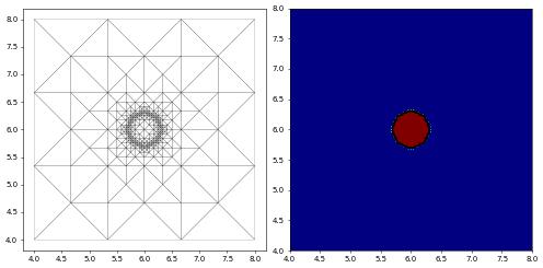
Let us start by plotting the initial state of the material, which is just a small circle in the centre.

from dune.fem.plotting import plotComponents
import matplotlib.pyplot as pyplot
from dune.fem.function import levelFunction, partitionFunction

# dummy vtk
def vtk():
    pass

We can construct a vtk writer that generates a sequence of files:

vtk = gridView.sequencedVTK("crystal", pointdata=[u_h],
         celldata=[levelFunction(gridView), partitionFunction(gridView)])

This can be for example used in a time loop. Simply adding vtk() in the loop will write files crystalXXXX.vtu where the sequence counter XXXX is automatically increased by one each time vtk() is called.

import matplotlib
matplotlib.rcParams.update({'font.size': 10})
matplotlib.rcParams['figure.figsize'] = [10, 5]
plotComponents(u_h, cmap=pyplot.cm.jet, show=[0], contours=[0.5],contourWidth=3)
vtk()

We set dt and the initial time t=0.

dt.value = 0.0005
t = 0.0

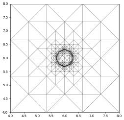
Finally, we set up the time loop and solve the problem - each time this cell is run the simulation will progress to the given endTime and then the result is shown. The simulation can be progressed further by rerunning the cell while increasing the endTime.

from dune.fem.plotting import plotPointData
u_h[0].plot(onlyContours=True,contours=[0.5], contourWidth=1, contourColor="black")
endTime = 0.1
while t < endTime:
    u_h_n.assign(u_h)
    scheme.solve(target=u_h)
    # print(t, gridView.size(0), end="\r")
    t += dt.value
    fem.mark(indicator,1.4,1.2,0,maxLevel)
    fem.adapt(u_h) # can also be a list or tuple of function to prolong/restrict
    fem.loadBalance(u_h) # can also be a list or tuple of function
    vtk()                # store result in sequence of vtk file
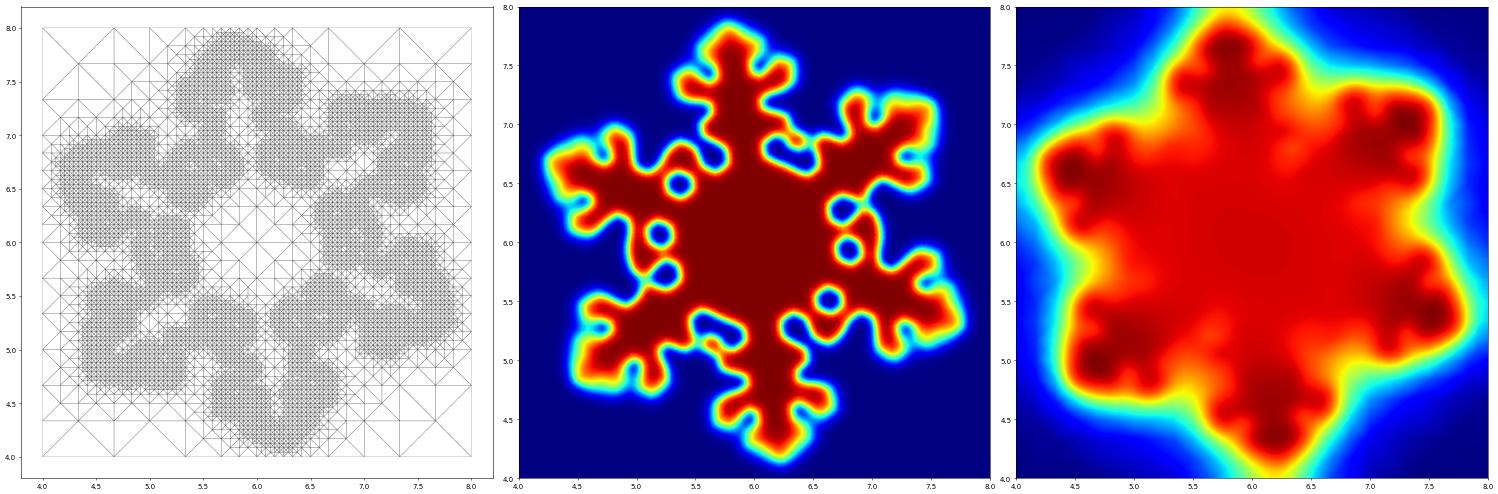
print()

fig = pyplot.figure(figsize=(30,10))
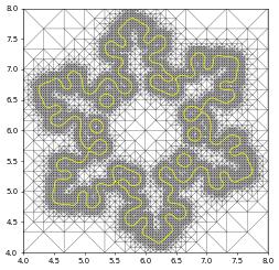
plotComponents(u_h, figure=fig)
u_h[0].plot(onlyContours=True,contours=[0.5], contourWidth=1, contourColor="yellow")

This page was generated from the notebook crystal_nb.ipynb and is part of the tutorial for the dune-fem python bindings