Mean Curvature Flow (revisited)
As discussed before we can simulate the shrinking of a sphere under mean curvature flow using a finite element approach based on the following time discrete approximation: \begin{align} \int_{\Gamma^n} \big( U^{n+1} - {\rm id}\big) \cdot \varphi + \tau \int_{\Gamma^n} \big( \theta\nabla_{\Gamma^n} U^{n+1} + (1-\theta) I \big) \colon\nabla_{\Gamma^n}\varphi =0~. \end{align} Here \(U^n\) parametrizes \(\Gamma(t^{n+1})\) over \(\Gamma^n:=\Gamma(t^{n})\), \(I\) is the identity matrix, \(\tau\) is the time step and \(\theta\in[0,1]\) is a discretization parameter.
If the initial surface \(\Gamma^0\) is a sphere of radius \(R_0\), the surface remains sphere and we have an exact formula for the evolution of the radius of the surface
To compare the accuracy of the surface approximation we compute an average radius of the discrete surface in each time step \(t^n\) using
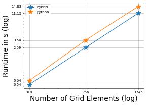
Computing \(R_h^n\) requires a grid traversal and a number of calls to interface methods on each element. Doing this on the Python side has a potential performance impact which we investigate here by comparing a pure python implementation with a hybrid approach where computing \(R_h^n\) is implemented in C++ using the dune.generator.algorithm functionality.
[1]:
import time, io
import pickle
import numpy
from matplotlib import pyplot as plt
from matplotlib.ticker import ScalarFormatter

from ufl import *
import dune.ufl
from dune.generator import algorithm
import dune.geometry as geometry
import dune.fem as fem

def plot(ct, ct2):
    fig, ax = plt.subplots()
    plt.loglog(ct[0][:], ct[1][:],'*-', markersize=15, label='hybrid')
    plt.loglog(ct2[0][:], ct2[1][:],'*-', markersize=15, label='python')
    plt.grid(True)
    for axis in [ax.xaxis, ax.yaxis]:
        axis.set_major_formatter(ScalarFormatter())
        axis.set_minor_formatter(ScalarFormatter())
    yticks = ax.yaxis.get_minor_ticks()
    for t in yticks:
        t.label1.set_visible(False)
    xticks = ax.xaxis.get_minor_ticks()
    for t in xticks:
        t.label1.set_visible(False)
    plt.yticks(numpy.append(ct[1], ct2[1]))
    plt.xticks(ct[0])
    plt.legend(loc="upper left")
    plt.xlabel('Number of Grid Elements (log)',fontsize=20)
    plt.gcf().subplots_adjust(bottom=0.17, left=0.16)
    plt.ylabel('Runtime in s (log)',fontsize=20)

# polynomial order of surface approximation
order = 2

# initial radius
R0 = 2.

# end time
endTime = 0.1
Main function for calculating the mean curvature flow of a given surface. If first argument is True the radius of the computed surface is computed using an algorithm implemented in C++ otherwise the computation is done in Python.
[2]:
def calcRadius(surface):
    R,vol = 0, 0
    for e in surface.elements:
        rule = geometry.quadratureRule(e.type, 4)
        for p in rule:
            geo = e.geometry
            weight = geo.volume * p.weight
            R   += geo.toGlobal(p.position).two_norm * weight
            vol += weight
    return R/vol

code = """
#include <dune/geometry/quadraturerules.hh>
template< class Surface >
double calcRadius( const Surface &surface ) {
  double R = 0, vol = 0.;
  for( const auto &entity : elements( surface ) ) {
    const auto& rule = Dune::QuadratureRules<double, 2>::rule(entity.type(), 4);
    for ( const auto &p : rule ) {
      const auto geo = entity.geometry();
      const double weight = geo.volume() * p.weight();
      R   += geo.global(p.position()).two_norm() * weight;
      vol += weight;
    }
  }
  return R/vol;
}
"""
switchCalcRadius = lambda use_cpp,surface: \
             algorithm.load('calcRadius', io.StringIO(code), surface) \
             if use_cpp else calcRadius
Timings for a number of different grid refinements is dumped to disk
[3]:
from dune.fem.view import geometryGridView as geoGridView
from dune.fem.space import lagrange as solutionSpace
from dune.fem.scheme import galerkin as solutionScheme
def calculate(use_cpp, gridView):
    # space on Gamma_0 to describe position of Gamma(t)
    space = solutionSpace(gridView, dimRange=gridView.dimWorld, order=order)
    u = TrialFunction(space)
    v = TestFunction(space)
    x = SpatialCoordinate(space)
    positions = space.interpolate(x, name="position")

    # space for discrete solution on Gamma(t)
    surface = geoGridView(positions)
    space = solutionSpace(surface, dimRange=surface.dimWorld, order=order)
    solution  = space.interpolate(x, name="solution")

    # set up model using theta scheme
    theta = 0.5   # Crank-Nicolson

    I = Identity(3)
    dt = dune.ufl.Constant(0,"dt")

    a = (inner(u - x, v) + dt * inner(theta*grad(u)
        + (1 - theta)*I, grad(v))) * dx

    scheme = solutionScheme(a == 0, space, solver="cg")

    Rexact = lambda t: numpy.sqrt(R0*R0 - 4.*t)
    radius = switchCalcRadius(use_cpp,surface)

    dt.value = 0.02

    numberOfLoops = 3
    times = numpy.zeros(numberOfLoops)
    errors = numpy.zeros(numberOfLoops)
    totalIterations = numpy.zeros(numberOfLoops, numpy.dtype(numpy.uint32))
    gridSizes = numpy.zeros(numberOfLoops, numpy.dtype(numpy.uint32))
    for i in range(numberOfLoops):
        positions.interpolate(x * (R0/sqrt(dot(x,x))))
        solution.interpolate(x)
        t = 0.
        error = abs(radius(surface)-Rexact(t))
        iterations = 0
        start = time.time()
        while t < endTime:
            info = scheme.solve(target=solution)
            # move the surface
            positions.assign(solution)
            # store some information about the solution process
            iterations += int( info["linear_iterations"] )
            t          += scheme.model.dt
            error       = max(error, abs(radius(surface)-Rexact(t)))
        print("time used:", time.time() - start)
        times[i] = time.time() - start
        errors[i] = error
        totalIterations[i] = iterations
        gridSizes[i] = gridView.size(2)
        if i < numberOfLoops - 1:
            gridView.hierarchicalGrid.globalRefine(1)
            dt.value /= 2
    eocs = numpy.log(errors[0:][:numberOfLoops-1] / errors[1:]) / numpy.log(numpy.sqrt(2))
    try:
        import pandas as pd
        keys = {'size': gridSizes, 'error': errors, "eoc": numpy.insert(eocs, 0, None), 'iterations': totalIterations}
        table = pd.DataFrame(keys, index=range(numberOfLoops),columns=['size', 'error', 'eoc', 'iterations'])
        print(table)
    except ImportError:
        print("pandas module not found so not showing table - ignored")
        pass
    return gridSizes, times
Compute the mean curvature flow evolution of a spherical surface. Compare computational time of a pure Python implementation and using a C++ algorithm to compute the radius of the surface for verifying the algorithm.
[4]:
# set up reference domain Gamma_0
results = []
from dune.alugrid import aluConformGrid as leafGridView
gridView = leafGridView("sphere.dgf", dimgrid=2, dimworld=3)
results += [calculate(True, gridView)]

gridView = leafGridView("sphere.dgf", dimgrid=2, dimworld=3)
results += [calculate(False, gridView)]
time used: 0.3493824005126953
time used: 1.8420426845550537
time used: 7.964749097824097
   size     error       eoc  iterations
0   318  0.001060       NaN          76
1   766  0.000605  1.619153         208
2  1745  0.000275  2.275142         420
time used: 0.6204028129577637
time used: 3.396092176437378
time used: 15.075105905532837
   size     error       eoc  iterations
0   318  0.001060       NaN          76
1   766  0.000605  1.619153         208
2  1745  0.000275  2.275142         420
Compare the hybrid and pure Python versions
[5]:
plot(results[0],results[1])
This page was generated from
the notebook mcf-algorithm_nb.ipynb
and is part of the tutorial for the dune-fem python bindings
![]()