Dual Weighted Reisdual Estimate (revisited)

In this problem we revisit the Re-entrant Corner Problem but instead of a classical residual estimator we use a dual weighted residual estimator. The aim will be to refine the grid to reduce the error at a given point.

Here we will consider the classic re-entrant corner problem, \begin{align*} -\Delta u &= f, && \text{in } \Omega, \\ u &= g, && \text{on } \partial\Omega, \end{align*} where the domain is given using polar coordinates, \begin{gather*} \Omega = \{ (r,\varphi)\colon r\in(0,1), \varphi\in(0,\Phi) \}~. \end{gather*} For the boundary condition \(g\), we set it to the trace of the function \(u\), given by \begin{gather*} u(r,\varphi) = r^{\frac{\pi}{\Phi}} \sin\big(\frac{\pi}{\Phi} \varphi \big) \end{gather*}

import matplotlib.pyplot as pyplot
import numpy
from dune.fem.plotting import plotPointData as plot
import dune.grid as grid
import dune.fem as fem
import dune.common as common
import dune.generator.algorithm as algorithm
from dune.fem.view import adaptiveLeafGridView as adaptiveGridView
from dune.fem.space import lagrange as solutionSpace
from dune.alugrid import aluConformGrid as leafGridView
from dune.ufl import DirichletBC
from dune.fem.function import gridFunction
from ufl import *
try: # this is needed to remain compatible with version 2022 of ufl
    from ufl import atan_2 as atan2
except:
    pass


# set the angle for the corner (0<angle<=360)
cornerAngle = 320.

# use a second order space
order = 2

We first define the domain and set up the grid and space. We need this twice - once for a computation on a globally refined grid and once for an adaptive one so we put the setup into a function:

We first define the grid for this domain (vertices are the origin and 4 equally spaced points on the unit sphere starting with (1,0) and ending at (cos(cornerAngle), sin(cornerAngle))

Next we define the model together with the exact solution.

def setup():
    vertices = numpy.zeros((8, 2))
    vertices[0] = [0, 0]
    for i in range(0, 7):
        vertices[i+1] = [numpy.cos(cornerAngle/6*numpy.pi/180*i),
                         numpy.sin(cornerAngle/6*numpy.pi/180*i)]
    triangles = numpy.array([[2,1,0], [0,3,2], [4,3,0],
                             [0,5,4], [6,5,0], [0,7,6]])
    domain = {"vertices": vertices, "simplices": triangles}
    gridView = adaptiveGridView( leafGridView(domain) )
    gridView.hierarchicalGrid.globalRefine(2)
    space = solutionSpace(gridView, order=order)

    from dune.fem.scheme import galerkin as solutionScheme
    u = TrialFunction(space)
    v = TestFunction(space)
    x = SpatialCoordinate(space)

    # exact solution for this angle
    Phi = cornerAngle / 180 * pi
    phi = atan2(x[1], x[0]) + conditional(x[1] < 0, 2*pi, 0)
    exact = dot(x, x)**(pi/2/Phi) * sin(pi/Phi * phi)
    a = dot(grad(u), grad(v)) * dx

    # set up the scheme
    laplace = solutionScheme([a==0, DirichletBC(space, exact, 1)], solver="cg",
            parameters={"linear.preconditioning.method":"jacobi"})
    uh = space.interpolate(0, name="solution")
    return uh, exact, laplace

uh, exact, laplace = setup()

Now we can setup the functional which will be \(J(v)=v(P)\) where \(P=(0.4,0.4)\) is some point in the computational domain at which we want to minimize the error. To compute the dwr estimator we need the solution to the dual problem with right hand side \(J(\varphi_i)\) for all basis functions \(\varphi_i\). This is not directly expressible in UFL and we therefore need to implement this either using some lower level functions on the space or using a small C++ function which we then export to Python.

from dune.fem.scheme import galerkin as solutionScheme
from dune.fem.utility import pointSample

spaceZ = solutionSpace(uh.space.gridView, order=order+1)
u = TrialFunction(spaceZ)
v = TestFunction(spaceZ)
x = SpatialCoordinate(spaceZ)
a = dot(grad(u), grad(v)) * dx
dual = solutionScheme([a==0,DirichletBC(spaceZ,0)], solver="cg")
z = spaceZ.interpolate(0, name="dual")
zh = uh.copy(name="dual_h")
point = common.FieldVector([0.4,0.4])
pointFunctional = z.copy("dual_rhs")
eh = gridFunction(abs(exact-uh),name="error", order=order+1)

def getFunctional(cpp=True):
    if cpp: # use the C++ version
        computeFunctional = algorithm.load("pointFunctional", "laplace-dwr.hh",
                                      point, pointFunctional, eh)
    else: # this is the equivalent implementation using the bindings
        def computeFunctional(point, pointFunctional, eh):
            space = pointFunctional.space
            en, xLoc = pointSample(space.gridView, point)
            phiVal = numpy.array( space.evaluateBasis(en, xLoc) )[:,0] # issue here with scalar function spaces
            idx = space.mapper()(en)
            lf = eh.localFunction()
            lf.bind(en)
            pointFunctional.as_numpy[ idx ] += phiVal
            return lf(xLoc)
    return computeFunctional

Here is the corresponding C++ code

#include <dune/fem/gridpart/common/entitysearch.hh>
#include <dune/fem/function/common/localcontribution.hh>
#include <dune/fem/function/localfunction/const.hh>
#include <dune/fem/common/bindguard.hh>

// Note: the coefficients of the functional will be ADDED to the storage of the functional
template <class Point, class Functional, class Error>
double pointFunctional(const Point &point, Functional &functional, Error &error)
{
  // first find the entity containing `point`
  typedef typename Functional::DiscreteFunctionSpaceType::GridPartType GridPartType;
  Dune::Fem::EntitySearch<GridPartType> search(functional.space().gridPart());
  const auto &entity = search(point);
  const auto localPoint = entity.geometry().local(point);

  // add the contributions from the basis functions to `functional`
  Dune::Fem::AddLocalContribution< Functional > wLocal( functional );
  {
    auto guard = Dune::Fem::bindGuard( wLocal, entity );
    typename Functional::RangeType one( 1 );
    wLocal.axpy(localPoint, one);
  }

  // in addition we also want to compute the value of `error` at `point`
  auto localError = constLocalFunction(error);
  localError.bind(entity);
  return localError.evaluate(localPoint)[0];
}

Next we define the actual estimator

from dune.fem.space import finiteVolume as estimatorSpace
from dune.fem.operator import galerkin as estimatorOp

fvspace = estimatorSpace(uh.space.gridView)
estimate = fvspace.interpolate([0], name="estimate")

u = TrialFunction(uh.space)
v = TestFunction(fvspace)
n = FacetNormal(fvspace)
estimator_ufl = abs(div(grad(u)))*abs(z-zh) * v * dx +\
                abs(inner(jump(grad(u)), n('+')))*abs(avg(z-zh)) * avg(v) * dS
estimator = estimatorOp(estimator_ufl)

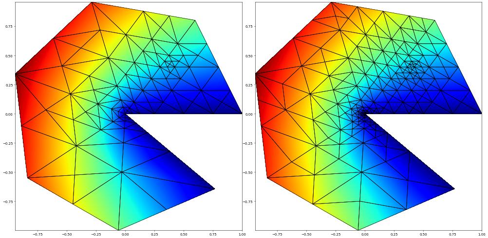
Let us solve over a loop (solve,estimate,mark) and plot the solutions side by side.

h1error = dot(grad(uh - exact), grad(uh - exact))

def compute(computeFunctional, tolerance):
    fig = pyplot.figure(figsize=(20,10))
    count = 0
    errorVector    = []
    estimateVector = []
    dofs           = []
    while True:
        laplace.solve(target=uh)
        if count%9 == 6:
            plot(uh, figure=(fig, 121), colorbar=False, linewidth=1)
        pointFunctional.clear()
        error = computeFunctional(point, pointFunctional,eh)
        dual.solve(target=z, rightHandSide=pointFunctional)
        zh.interpolate(z)
        estimator(uh, estimate)
        eta = sum(estimate.dofVector)
        dofs           += [uh.space.size]
        errorVector    += [error]
        estimateVector += [eta]
        if count%3 == 2:
            print(count, ": size=", uh.space.gridView.size(0), "estimate=", eta, "error=", error)
        if eta < tolerance:
            break
        marked = fem.mark(estimate,eta/uh.space.gridView.size(0))
        fem.adapt(uh) # can also be a list or tuple of function to prolong/restrict
        fem.loadBalance(uh)
        count += 1
    plot(uh, figure=(fig, 122), colorbar=False, linewidth=1)

We first use a version based entirely on the available binding:

compute( getFunctional(cpp=False), tolerance=1e-4 )

2 : size= 49 estimate= 0.002172772767494346 error= 0.0013543219723589628
5 : size= 115 estimate= 0.0005316985104321773 error= 0.0005407738706248444
8 : size= 217 estimate= 0.00016016431030722942 error= 0.00015909061408719838

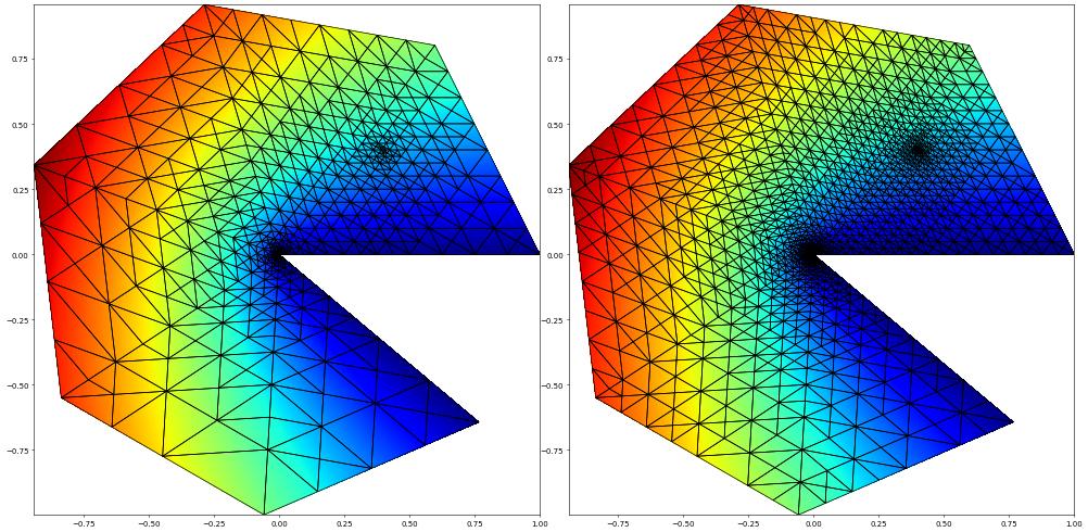
We repeat the same simulation providing part of the code in a cpp code snippet. We reduce the tolerance a bit to get a more accurate results. Note that this is just to demonstrate the concept of using the algorithm function, the same result could have been achieved using the binding code used previously by reducing the tolerance in the first call to compute.

compute( getFunctional(cpp=True), tolerance=1e-6 )

2 : size= 481 estimate= 3.553725447796442e-05 error= 3.468638369830135e-05
5 : size= 873 estimate= 1.172940917180334e-05 error= 1.153418375043902e-05
8 : size= 1527 estimate= 3.73406322670498e-06 error= 3.576365975033191e-06
11 : size= 2736 estimate= 1.237247482000582e-06 error= 1.1891840905331463e-06

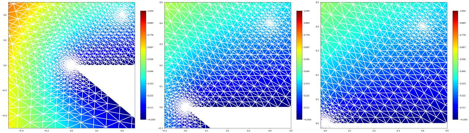
Let’s take a close up look of the refined region around the point of interest and the origin:

pyplot.close('all')
fig = pyplot.figure(figsize=(30,10))
plot(uh, figure=(fig, 131), xlim=(-0.5, 0.5), ylim=(-0.5, 0.5),
        gridLines="white", colorbar={"shrink": 0.75}, linewidth=2)
plot(uh, figure=(fig, 132), xlim=(-0.1, 0.5), ylim=(-0.1, 0.5),
        gridLines="white", colorbar={"shrink": 0.75}, linewidth=2)
plot(uh, figure=(fig, 133), xlim=(-0.02, 0.5), ylim=(-0.02, 0.5),
        gridLines="white", colorbar={"shrink": 0.75}, linewidth=2)

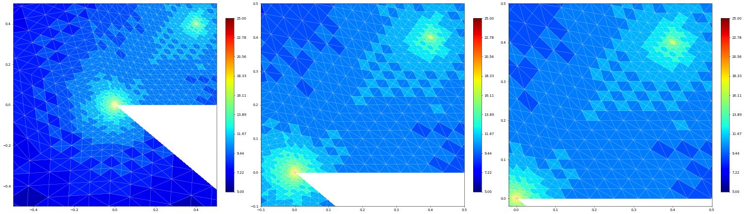
fig = pyplot.figure(figsize=(30,10))
from dune.fem.function import levelFunction
levels = levelFunction(uh.space.gridView)
plot(levels, figure=(fig, 131), xlim=(-0.5, 0.5), ylim=(-0.5, 0.5),
        gridLines="white", colorbar={"shrink": 0.75})
plot(levels, figure=(fig, 132), xlim=(-0.1, 0.5), ylim=(-0.1, 0.5),
        gridLines="white", colorbar={"shrink": 0.75})
plot(levels, figure=(fig, 133), xlim=(-0.02, 0.5), ylim=(-0.02, 0.5),
        gridLines="white", colorbar={"shrink": 0.75})

This page was generated from the notebook laplace-dwr-algorithm_nb.ipynb and is part of the tutorial for the dune-fem python bindings