The main concepts of our virtual element implementation is provided in [DH21] where we focus on the fourth order problems but the second order problems are discussed there as well.

Elliptic Problems

We first consider an elliptic problem with varying coefficients and Dirichlet boundary conditions \begin{align*} -\nabla D(x)\nabla u + \mu(x) u &= f, && \text{in } \Omega, \\ u &= g, && \text{on } \partial\Omega, \end{align*} with \(\Omega=[-\frac{1}{2},1]^2\) and choosing the forcing and the boundary conditions so that the exact solution is equal to \begin{align*} u(x,y) &= xy\cos(\pi xy) \end{align*}

First some setup code:

try:
    import dune.vem
except:
    print("This example needs 'dune.vem' - skipping")
    import sys
    sys.exit(0)

from matplotlib import pyplot
import numpy
from dune.grid import cartesianDomain, gridFunction
from dune.fem.plotting import plotPointData as plot
from dune.fem.function import discreteFunction
from dune.fem import integrate
import dune.fem

from ufl import *
import dune.ufl

We use a grid build up of voronoi cells around \(50\) random points in the interval \([-\frac{1}{2},1]\times [-\frac{1}{2},1]\) using 100 iterations of Lloyd’s algorithm to improve the quality of the grid.

polyGrid = dune.vem.polyGrid( dune.vem.voronoiCells([[-0.5,-0.5],[1,1]], 50, lloyd=100) )

One can also use a standard simplex or cube grid, e.g., polyGrid = dune.vem.polyGrid( cartesianDomain([-0.5,-0.5],[1,1],[10,10]), cubes=False)

In general we can construct a polygrid by providing a dictionary with the vertices and the polygons. The voronoiCells function creates such a dictionary using random seeds to generate voronoi cells which are cut off using the provided cartesianDomain. The seeds can be provided as list of points as second argument:

voronoiCells(constructor, towers, fileName=None, load=False):

If a fileName is provided the seeds will be written to disc or if that file exists they will be loaded from that file if load=True, to make results reproducible.

As an example an output of voronoiCells(constructor,5) is

{'polygons': [ [4, 5, 2, 3], [ 8, 10,  9,  7], [7, 9, 1, 3, 4],
               [11, 10,  8,  0], [8, 0, 6, 5, 4, 7] ],
 'vertices': [ [ 0.438, 1.  ],    [ 1. , -0.5 ],
               [-0.5, -0.5  ],    [ 0.923, -0.5 ],
               [ 0.248,  0.2214], [-0.5,  0.3027],
               [-0.5,  1. ],      [ 0.407,0.4896],
               [ 0.414,  0.525],  [ 1.,  0.57228],
               [ 1., 0.88293],    [ 1.,  1. ] ] }

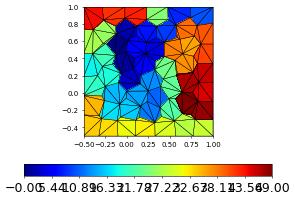
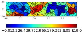
Let’s take a look at the grid with the 50 polygons triangulated

indexSet = polyGrid.indexSet
@gridFunction(polyGrid, name="cells")
def polygons(en,x):
    return polyGrid.hierarchicalGrid.agglomerate(indexSet.index(en))
polygons.plot(colorbar="horizontal")

The vem space is now setup in exactly the same way as usual but the type of space constructed is defined by the final argument which defines the moments used on the subentities of a given codimension. So testSpaces=[-1,order-1,order-2] means: use no vertex values (-1), order-1 moments on the edges and order-2 moments in the inside. So this gives us a non-conforming space for second order problems - while using testSpaces=[0,order-2,order-2] defines a conforming space.

order = 3
space = dune.vem.vemSpace( polyGrid, order=order, storage="numpy",
                           testSpaces=[-1,order-1,order-2])

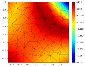
Now we define the model starting with the exact solution:

x = SpatialCoordinate(space)
u = TrialFunction(space)
v = TestFunction(space)

exact = x[0]*x[1] * cos(pi*x[0]*x[1])

massCoeff = 1+sin(dot(x,x))       # factor for mass term
diffCoeff = 1-0.9*cos(dot(x,x))   # factor for diffusion term

a = (diffCoeff*inner(grad(u),grad(v)) + massCoeff*dot(u,v) ) * dx

# finally the right hand side and the boundary conditions
b = (-div(diffCoeff*grad(exact)) + massCoeff*exact ) * v * dx
dbc = [dune.ufl.DirichletBC(space, exact, i+1) for i in range(4)]

Finally, we can construct the solver passing in the space the pde description and arguments for stabilization:

parameters = {"newton.linear.tolerance": 1e-12,
              "newton.linear.preconditioning.method": "jacobi",
              "penalty": 10*order*order,  # for the dg schemes
              "newton.linear.verbose": False,
              "newton.verbose": False
              }
df = space.interpolate(0,name="solution")
scheme = dune.vem.vemScheme( [a==b, *dbc], space, solver="cg",
                             gradStabilization=diffCoeff,
                             massStabilization=massCoeff,
                             parameters=parameters )
info = scheme.solve(target=df)
print("size of space:",space.size,flush=True)
df.plot()

size of space: 603

Repeating the same test with a H^1-conforming space

space = dune.vem.vemSpace( polyGrid, order=order, storage="numpy",
                           testSpaces=[0,order-2,order-2])
df = space.interpolate(0,name="solution")
scheme = dune.vem.vemScheme( [a==b, *dbc], space, solver="cg",
                             gradStabilization=diffCoeff,
                             massStabilization=massCoeff,
                             parameters=parameters )
info = scheme.solve(target=df)
print("size of space:",space.size,flush=True)
df.plot()

size of space: 554

The Vem spaces have an additional method :code:diameters which returns estimation of the polygon sizes. Note that for technical reasons this is at the time of writing not available on the grid itself. A estimate of the minimum and the maximum bounding box diameters are returned. Note that this is just an estimate of the actual polygon diameters.

print("Polygon diameters:",space.diameters())

Polygon diameters: (0.20497517186795178, 0.26902334164593067)

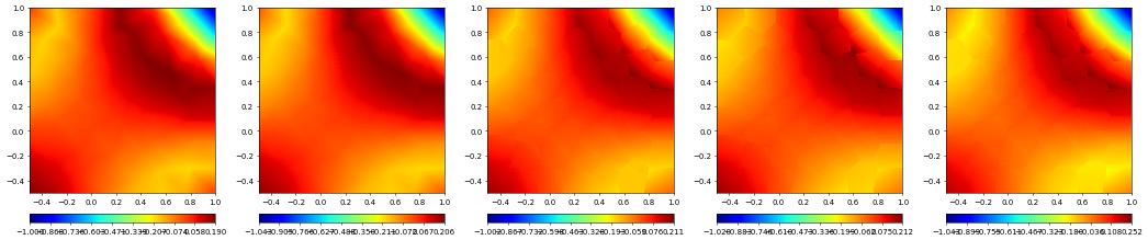
We can compare different method, e.g., a lagrange/dg scheme (on the the subtriangulation), a bounding box dg method and conforming/non conforming VEM:

methods = [ ### "[legend,space,scheme,spaceKwargs,schemeKwargs]"
            ["lagrange",
             dune.fem.space.lagrange,dune.fem.scheme.galerkin,{},{}],
            ["dg",
             dune.fem.space.dgonb, dune.fem.scheme.dg,  {}, {"penalty":diffCoeff}],
            ["vem-conforming",
             dune.vem.vemSpace,    dune.vem.vemScheme,
                {"testSpaces":[0,order-2,order-2]},  # conforming vem space
                {"gradStabilization":diffCoeff, "massStabilization":massCoeff}],
            ["vem-nonconforming",
             dune.vem.vemSpace,    dune.vem.vemScheme,
                 {"testSpaces":[-1,order-1,order-2]},  # non-conforming vem space
                 {"gradStabilization":diffCoeff, "massStabilization":massCoeff}],
            ["bb-dg",
             dune.vem.bbdgSpace,   dune.vem.bbdgScheme, {}, {"penalty":diffCoeff}],
   ]

We now define a function to compute the solution and the \(L^2,H^1\) error given a grid and a space

def compute(grid, space,spaceArgs, schemeName,schemeArgs):
    space = space( grid, order=order, **spaceArgs )
    df = space.interpolate(0,name="solution")
    scheme = schemeName( [a==b, *dbc], space, solver="cg", **schemeArgs,
                         parameters=parameters )
    info = scheme.solve(target=df)

    # compute the error
    edf = exact-df
    err = [inner(edf,edf),
           inner(grad(edf),grad(edf))]
    errors = [ numpy.sqrt(e) for e in integrate(err) ]

    return df, errors, info

Finally we iterate over the requested methods and solve the problems

fig = pyplot.figure(figsize=(5*len(methods),10))
figPos = 111+10*len(methods)
for i,m in enumerate(methods):
    dfs,errors,info = compute(polyGrid, m[1],m[3], m[2],m[4])
    print("method (",m[0],"):",
          "dofs: ",dfs.space.size,
          "L^2: ", errors[0], "H^1: ", errors[1],
          info["linear_iterations"], flush=True)
    dfs.plot(figure=(fig,figPos+i), gridLines=None, colorbar="horizontal")

method ( lagrange ): dofs:  829 L^2:  0.00014798685281600801 H^1:  0.0068585822225753715 273
method ( dg ): dofs:  1750 L^2:  0.0001384939266553391 H^1:  0.00670817860418124 2892
method ( vem-conforming ): dofs:  554 L^2:  0.0006059720464613047 H^1:  0.013720699134208434 135
method ( vem-nonconforming ): dofs:  603 L^2:  0.0004375885012392981 H^1:  0.012997824243772046 127
method ( bb-dg ): dofs:  500 L^2:  0.0003879437501581428 H^1:  0.01364357273229881 381

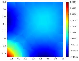
Nonlinear Elliptic Problem

We can easily set up a non linear problem

space = dune.vem.vemSpace( polyGrid, order=1, conforming=True )
u = TrialFunction(space)
v = TestFunction(space)
x = SpatialCoordinate(space)
exact = (x[0] - x[0]*x[0] ) * (x[1] - x[1]*x[1] )
Dcoeff = lambda u: 1.0 + u**2
a = (Dcoeff(u) * inner(grad(u), grad(v)) ) * dx
b = -div( Dcoeff(exact) * grad(exact) ) * v * dx
dbcs = [dune.ufl.DirichletBC(space, exact, i+1) for i in range(4)]
scheme = dune.vem.vemScheme( [a==b, *dbcs], space, gradStabilization=Dcoeff(u),
                             solver="cg", parameters=parameters)
solution = space.interpolate(0, name="solution")
info = scheme.solve(target=solution)
edf = exact-solution
errors = [ numpy.sqrt(e) for e in
           integrate([inner(edf,edf),inner(grad(edf),grad(edf))]) ]
print("non linear problem:", errors )
solution.plot(gridLines=None)

non linear problem: [0.008408963250176047, 0.1480707362296293]

Linear Elasticity

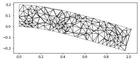
Next we solve a linear elasticity equation using a conforming VEM space:

First we setup the domain

L, W = 1, 0.2

beamGrid = dune.vem.polyGrid( dune.vem.voronoiCells([[0,0],[L,W]], 120) )
indexSet = beamGrid.indexSet
@gridFunction(beamGrid, name="cells")
def polygons(en,x):
    return beamGrid.hierarchicalGrid.agglomerate(indexSet.index(en))
polygons.plot(colorbar="horizontal")

# instead of providing the moments we can simply add a parameter 'conforming' to construct the H^1-conforming space
space = dune.vem.vemSpace( beamGrid, order=2, dimRange=2, conforming=True)

# some model constants
mu = 1
rho = 1
delta = W/L
gamma = 0.4*delta**2
beta = 1.25
lambda_ = beta
g = gamma

# clamped boundary on the left
x = SpatialCoordinate(space)
dbc = dune.ufl.DirichletBC(space, as_vector([0,0]), x[0]<1e-10)

# Define strain and stress
def epsilon(u):
    return 0.5*(nabla_grad(u) + nabla_grad(u).T)
def sigma(u):
    return lambda_*nabla_div(u)*Identity(2) + 2*mu*epsilon(u)

# Define the variational problem
u = TrialFunction(space)
v = TestFunction(space)
f = dune.ufl.Constant((0, -rho*g))
a = inner(sigma(u), epsilon(v))*dx
b = dot(as_vector([0,-rho*g]),v)*dx

# Compute solution
displacement = space.interpolate([0,0], name="displacement")
scheme = dune.vem.vemScheme( [a==b, dbc], space,
        gradStabilization = as_vector([lambda_+2*mu, lambda_+2*mu]),
        solver="cg", parameters=parameters )
info = scheme.solve(target=displacement)

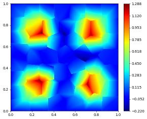
Show the magnitude of the displacement field, stress and the deformed beam

fig = pyplot.figure(figsize=(20,10))
displacement.plot(gridLines=None, figure=(fig, 121), colorbar="horizontal")
s = sigma(displacement) - (1./3)*tr(sigma(displacement))*Identity(2)
von_Mises = sqrt(3./2*inner(s, s))
plot(von_Mises, gridView=beamGrid, gridLines=None, figure=(fig, 122), colorbar="horizontal")

Finally we plot the deformed beam

from dune.fem.view import geometryGridView
position = space.interpolate( x+displacement, name="position" )
beam = geometryGridView( position )
beam.plot()

Fourth order problem

As final example we solve some fourth order PDEs using a non-conforming VEM space for \(H^2\) functions. To construct the space we just need to define a suitable ‘moments’ vector to construct a suitable space for \(H^2\) problems.

ncC1testSpaces = [ [0], [order-3,order-2], [order-4] ]

We test the method using a biharmonic problem. \begin{align*} -\Delta^2 u &= f, && \text{in } \Omega, \\ u &= g, && \text{on } \partial\Omega, \\ \nabla u.n &= 0, && \text{on } \partial\Omega, \end{align*}

Note: For function with continuous derivatives we have laplace(u)laplace(v)dx = inner(u,v)*dx as can be seen by using integration by parts on the mixed terms on the right and using continuity of u,v. For the non-conforming spaces we don’t have continuity of the derivatives so the equivalence does not hold and one should use the right hand side directly to obtain a coercive bilinear form w.r.t. the norm on \(H^2\) (the left is not a norm in this case). For computing the forcing term ‘b’ both formula are fine since ‘exact’ is smooth enough.

polyGrid = dune.vem.polyGrid( dune.vem.voronoiCells([[0,0],[1,1]], 50, lloyd=100) )
space = dune.vem.vemSpace( polyGrid, order=order, testSpaces=ncC1testSpaces)

x = SpatialCoordinate(space)
exact = sin(2*pi*x[0])**2*sin(2*pi*x[1])**2

laplace = lambda w: div(grad(w))
H = lambda w: grad(grad(w))
u = TrialFunction(space)
v = TestFunction(space)
a = ( inner(H(u),H(v)) ) * dx

# finally the right hand side and the boundary conditions
b = laplace(laplace(exact)) * v * dx
dbcs = [dune.ufl.DirichletBC(space, [0], i+1) for i in range(4)]

scheme = dune.vem.vemScheme( [a==b, *dbcs], space, hessStabilization=1,
                             solver="cg", parameters=parameters )

# solution = space.interpolate(0, name="solution") # issue here for C^1 spaces
solution = discreteFunction(space, name="solution")
info = scheme.solve(target=solution)
edf = exact-solution
errors = [ numpy.sqrt(e) for e in
           integrate([inner(edf,edf),inner(grad(edf),grad(edf))]) ]
print("bi-laplace errors:", errors )
solution.plot(gridLines=None)

bi-laplace errors: [0.089261909447782, 1.0111552233833234]

This page was generated from the notebook vemdemo_nb.ipynb and is part of the tutorial for the dune-fem python bindings