Introduction

A Laplace problem

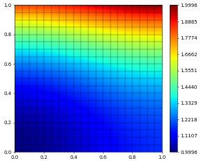
As an introduction we will solve \begin{equation} -\triangle u + u = f \end{equation} in \(\Omega=[0,1]^2\), where \(f=f(x)\) is a given forcing term. On the boundary we prescribe Neumann boundary \(\nabla u\cdot n = 0\).

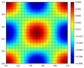
We will solve this problem in variational form \(a(u,v) = l(v)\) with \begin{equation} a(u,v) := \int_\Omega \nabla u\cdot\nabla v + uv~,\qquad l(v) := \int_\Omega fv~. \end{equation} We choose \(f=(8\pi^2+1)\cos(2\pi x_1)\cos(2\pi x_2)\) so that the exact solution is \begin{align*} u(x) = \cos(2\pi x_1)\cos(2\pi x_2) \end{align*}

We first need to setup a tessellation of \(\Omega\). We use a Cartesian grid with a 20 cells in each coordinate direction

import numpy as np

from dune.grid import structuredGrid
gridView = structuredGrid([0, 0], [1, 1], [20, 20])

Note

In the following we will often use the term gridView instead of grid. The details of what a gridView is together with some other central concepts is provided in the next section.

Tip

An overview of available approaches to construct a grid can be found here.

Next we define a linear Lagrange Finite-Element space over that grid and setup a discrete function which we will store the discrete solution to our PDE

from dune.fem.space import lagrange
space = lagrange(gridView, order=1)
u_h   = space.interpolate(0, name='u_h')

We define the mathematical problem using ufl

from ufl import (TestFunction, TrialFunction, SpatialCoordinate,
                 dx, grad, inner, dot, sin, cos, pi )
x = SpatialCoordinate(space)
u = TrialFunction(space)
v = TestFunction(space)

f = (8*pi**2+1) * cos(2*pi*x[0])*cos(2*pi*x[1])
a = ( inner(grad(u),grad(v)) + u*v ) * dx
l = f*v * dx

Now we can assemble the matrix and the right hand side

from dune.fem import assemble
mat,rhs = assemble(a==l)

We solve the resulting linear system of equations \(Ay=b\) using scipy. To this end it is straightforward to expose the underlying data structures of mat,rhs and u_h using the as_numpy attribute.

from scipy.sparse.linalg import spsolve as solver

A = mat.as_numpy
b = rhs.as_numpy
y = u_h.as_numpy
y[:] = solver(A,b)

Note the y[:] which guarantees that the result from the solver is stored in the same buffer used for the discrete function. Consequently, no copying is required.

Tip

More details on how to use Scipy will be given later in the tutorial. Other linear solver backends are also available, e.g., PETSc and PETSc4py can also be used.

That’s it - to see the result we plot it using matplotlib

u_h.plot()

Since in this case the exact solution is known, we can also compute the \(L^2\) and \(H^1\) errors to see how good our approximation actually is

from dune.fem import integrate
exact = cos(2*pi*x[0])*cos(2*pi*x[1])
e_h = u_h-exact
squaredErrors = integrate([e_h**2,inner(grad(e_h),grad(e_h))])
print("L^2 and H^1 errors:",[np.sqrt(e) for e in squaredErrors])

L^2 and H^1 errors: [0.004816749930263432, 0.40259995183954644]

Note

The assemble function can be used to assemble bilinear forms as shown above, linear forms (functionals) as shown further down, and to compute scalar integrals. So we could compute the \(L^2\) error using assemble(e_h**2*dx). We use the integrate function above since it allows to integrate vector valued expressions which is more efficient than calling assemble multiple times. Using the assemble function with ‘a==l’ and ‘a-l==0’ produces the same result.

Tip

Both assemble and integrate take extra arguments gridView and order. The latter allows to fix the order of the quadrature used to integrate a function - if it is not provided (None) a reasonable order is determined heuristically. The gridView argument is required in cases where the gridView can not be determined from the ufl expression.

In the above example gridView can be extracted from the discrete function u_h which is part of the expression for e_h. Consider instead the following example where the gridView has to be provided to the integrate method

print("average:",integrate(exact,gridView=gridView) )
# since the integrand is scalar, the following is equivalent:
print("average:",assemble(exact*dx,gridView=gridView) )

average: 1.5720931501039814e-17
average: 1.5720931501039814e-17

Laplace equation with Dirichlet boundary conditions

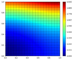
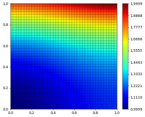
We consider the scalar boundary value problem \begin{align*} -\triangle u &= f & \text{in}\;\Omega:=(0,1)^2 \\ \nabla u\cdot n &= g_N & \text{on}\;\Gamma_N \\ u &= g_D & \text{on}\;\Gamma_D \end{align*} and \(f=f(x)\) is some forcing term. For the boundary conditions we set \(\Gamma_D=\{0\}\times[0,1]\) and take \(\Gamma_N\) to be the remaining boundary of \(\Omega\).

We will solve this problem in variational form \begin{align*} \int \nabla u \cdot \nabla \varphi \ - \int_{\Omega} f(x) \varphi\ dx - \int_{\Gamma_N} g_N(x) v\ ds = 0. \end{align*}

We choose \(f,g_N,g_D\) so that the exact solution is \begin{align*} u(x) = \left(\frac{1}{2}(x_1^2 + x_2^2) - \frac{1}{3}(x_1^3 - x_2^3)\right) + 1~. \end{align*}

Tip

More general boundary conditions are discussed in a later section.

The setup of the model using ufl is very similar to the previous example but we need to include the non trivial Neumann boundary conditions:

from ufl import conditional, FacetNormal, ds, div

exact = 1/2*(x[0]**2+x[1]**2) - 1/3*(x[0]**3 - x[1]**3) + 1
a   = dot(grad(u), grad(v)) * dx
f   = -div( grad(exact) )
g_N = grad(exact)
n   = FacetNormal(space)
l   = f*v*dx + dot(g_N,n)*conditional(x[0]>=1e-8,1,0)*v*ds

With the model described as a ufl form, we can again assemble the system matrix and right hand side using dune.fem.assemble. To take the Dirichlet boundary conditions into account we construct an instance of dune.ufl.DirichletBC that described the values to use and the part of the boundary to apply them to. This is then passed into the assemble function:

from dune.ufl import DirichletBC
dbc = DirichletBC(space,exact,x[0]<=1e-8)
mat,rhs = assemble([a==l,dbc])

Solving the linear system of equations, plotting the solution, and computing the error is now identical to the previous example:

u_h.as_numpy[:] = solver(mat.as_numpy, rhs.as_numpy)
u_h.plot()
e_h = u_h-exact
squaredErrors = integrate([e_h**2,inner(grad(e_h),grad(e_h))])
print("L^2 and H^1 errors:",[np.sqrt(e) for e in squaredErrors])

L^2 and H^1 errors: [0.000492922796816225, 0.031176023550870714]

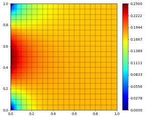
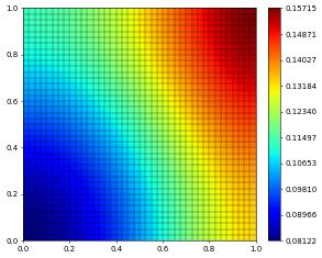
It is straightforward to solve a problem with a different right hand side and different boundary values. Assuming the type of the boundary conditions remains the same, the system matrix does not change we only need to reassemble the right hand side:

l   = conditional(dot(x,x)<0.1,1,0)*v*dx
dbc = DirichletBC(space,x[1]*(1-x[1]),x[0]<=1e-8)
rhs = assemble([l,dbc])
u_h.as_numpy[:] = solver(mat.as_numpy, rhs.as_numpy)
u_h.plot()

A non-linear elliptic problem

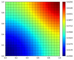
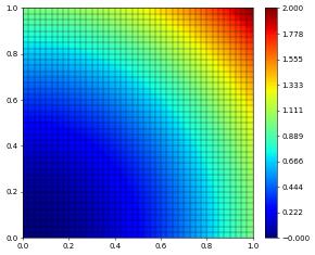
It is very easy to solve a non-linear elliptic problem with very few changes to the above code. We will demonstrate this using the PDE \begin{equation} -\triangle u + m(u) = f \end{equation} in \(\Omega=[0,1]^2\), where again \(f=f(x)\) is a given forcing term and \(m=m(u)\) is some non-linearity. On the boundary we still prescribe Neumann boundary \(\nabla u\cdot n = 0\).

We will solve this problem in variational form \begin{equation} \int_\Omega \nabla u\cdot\nabla v + m(u)v = \int_\Omega fv~. \end{equation} We use \(f(x)=|x|^2\) as forcing and choose \(m(u) = (1+u)^2u\). Most of the code is identical to the linear case, we can use the same grid, discrete lagrange space, and the discrete function u_h. The model description using ufl is also very similar

a = ( inner(grad(u),grad(v)) + (1+u)**2*u*v ) * dx
l = dot(x,x)*v * dx

To solve the non-linear problem we need to use something like a Newton solver. We could use the implementation available in Scipy but dune-fem provides so called schemes that have a solve method which can handle both linear and non-linear models.

Note

The default solver is based on a Newton-Krylov solver using a gmres method to solve the intermediate linear problems.

Since the problem we are considering is symmetric we can use a cg method which we do during construction of the scheme:

from dune.fem.scheme import galerkin as solutionScheme
scheme = solutionScheme(a == l, solver='cg')
u_h.clear() # set u_h to zero as initial guess for the Newton solver
info = scheme.solve(target=u_h)

Tip

These schemes provide options for solving PDEs for writing your own solvers, accessing degrees of freedom on the boundary etc. A description of the API is given here and example usage is available in the sections on the use of internal solvers and external solvers. A list of solvers, preconditioners, and parameters is available here.

That’s it - we can plot the solution again - we don’t know the exact solution so we can’t compute any errors in this case. In addition the info structure returned by the solve method gives some information on the solver like number of iterations required

print(info)
u_h.plot()

{'converged': True, 'iterations': 5, 'linear_iterations': 250, 'timing': [0.007600417, 0.003880561, 0.003719856]}

Let’s complete this discussion by looking at the experimental order of convergence (EOC) of our approximation. For this we add a forcing that leads to the problem having the prescribed solution \begin{align*} u(x,y) = \left(\frac{1}{2}(x^2 + y^2) - \frac{1}{3}(x^3 - y^3)\right) + 1 \end{align*}

exact = 1/2*(x[0]**2+x[1]**2) - 1/3*(x[0]**3 - x[1]**3) + 1
a  = ( inner(grad(u),grad(v)) + (1+u)**2*u*v ) * dx
bf = (-div(grad(exact)) + (1+exact)**2*exact) * v * dx
bg = dot(grad(exact),n)*v*ds
scheme = solutionScheme(a == bf+bg, solver="cg")

errors = 0,0
loops = 2
for eocLoop in range(loops):
    u_h.interpolate(0)
    info = scheme.solve(target=u_h)
    errors_old = errors
    l2error, h1error = dot(u_h-exact, u_h-exact), dot(grad(u_h-exact), grad(u_h-exact))
    errors = [np.sqrt(e) for e in integrate([l2error,h1error])]
    if eocLoop == 0:
        eocs = ['-','-']
    else:
        eocs = [ round(np.log(e/e_old)/np.log(0.5),2) for e,e_old in zip(errors,errors_old) ]
    print("step:", eocLoop, ", size:", gridView.size(0))
    print("\t\t L^2, H^1 error:",'{:0.5e}, {:0.5e}'.format(*errors),", eocs =", eocs)
    print("\t\t solver info=",info)
    u_h.plot()
    if eocLoop < loops-1:
        gridView.hierarchicalGrid.globalRefine(1)

step: 0 , size: 400
                 L^2, H^1 error: 2.16373e-04, 3.11774e-02 , eocs = ['-', '-']
                 solver info= {'converged': True, 'iterations': 8, 'linear_iterations': 433, 'timing': [0.012410766, 0.006010214999999999, 0.006400551000000001]}

step: 1 , size: 1600
                 L^2, H^1 error: 5.40907e-05, 1.55899e-02 , eocs = [2.0, 1.0]
                 solver info= {'converged': True, 'iterations': 8, 'linear_iterations': 789, 'timing': [0.058403466, 0.024546358, 0.033857108]}

Using Constant parameters and grid functions in PDEs

Every time we call assemble or construct a new scheme as show above, some code must be compiled which leads to some extra cost. In time critical points of the simulation, e.g., in loops, this extra cost is not acceptable. To avoid recompilation general grid functions and placeholders for scalar or vector valued constants can be used within the ufl forms. In the next section we will give a full example for this in the context of a time dependent problems.

As a simple introduction we consider a linear version of the elliptic problem considered previously

\[-\varepsilon \triangle u(x) + m(x) u(x) = f(x)\]

with Neuman boundary conditions. We also added a real valued constant \(\varepsilon\) and we want to able to change \(m\) easily. Assuming \(\bar{u}\) is the exact solution of the non-linear elliptic problem from above then \(\bar{u}\) will also solve the above equation if \(\varepsilon=1\) and we chose \(m(x) = (1+\bar{u})^2\). We will use the discrete solution \(u_h\) from above, which is an approximation to \(\bar{u}\) and chose \(m(x) = (1+u_h)^2\). Later we want to solve the same linear problem but with \(\varepsilon=0\) and \(m(x)=1\) so that we are simply looking at the \(L^2\) projection of \(f\):

\[\int_\Omega uv = \int_\Omega fv~.\]

Although the problem is linear and we could just use dune.fem.assemble and Scipy to solve it, we will again use a scheme instead. Details on schemes and operators will be provided in the following section. For this example the important characteristic of a scheme is that we can still access some information contained in the underlying UFL form, e.g., the Constants used. This allows us to change these efficiently during the simulation as shown below.

from dune.ufl import Constant

epsilon = Constant(1,name="eps")   # start with epsilon=1
x,u,v   = SpatialCoordinate(space), TrialFunction(space), TestFunction(space)
f       = dot(x,x)
a       = epsilon*dot(grad(u), grad(v)) * dx + (1+u_h)**2*u*v * dx
b       = f*v*dx

scheme = solutionScheme(a == b, solver='cg')
w_h    = space.interpolate(0,name="w_h")
scheme.solve(target = w_h)
w_h.plot()

from dune.fem.operator import galerkin
op = galerkin(a == b)

Note that since \(\varepsilon=1\) and we use the previously computed approximation \(u_h\) the new discrete function \(w_h\) is close to \(u_h\).

We can print the value of a Constant with name foo either via scheme.model.foo or using the value on the Constant itself. We can change the value using the same attribute. See the discussion at the end of section on operators and schemes in the concepts chapter for more detail on these two approaches.

print(scheme.model.eps, epsilon.value)
epsilon.value = 0                          # change to the problem which matches our exact solution
print(scheme.model.eps, epsilon.value)

1.0 1.0
0.0 0.0

To switch to a standard \(L^2\) projection we will also change \(m=(1+u_h)^2\) to \(m\equiv 1\). This can be easily done by changing \(u_h\) to be zero everywhere. This can be either done using u_h.interpolate(0) or by using u_h.clear().

u_h.interpolate(0)
scheme.solve(target = w_h)
w_h.plot()

Tip

A wide range of problems a covered in the further examples section. In the next section we explain the main concepts we use to solve PDE using finite-element approximations which we end with a solution to a non-linear time-dependent problem using the Crank-Nicolson method in time.

This page was generated from the notebook dune-fempy_nb.ipynb and is part of the tutorial for the dune-fem python bindings