General Concepts (with a time dependent problem)

In the following we introduce how to construct and use the basic components of a finite element method ending with solving a heat equation. The required steps are:

constructing a tessellation of the computational domain (hierarchical grid and grid view)
working with functions defined over the grid (grid functions)
setting up discrete spaces and discrete functions
defining the mathematical model to solve (ufl)
solving the (non linear) system arising from the discretization of the model by the Galerkin method (scheme)

Setting up the Grid

Note

The goal of a Dune grid or hierarchical grid is to provide an interface to describe subdivisions (entities or elements for codim 0) of the computational domain \(\Omega\) in a generic way. In the following this is referred to as hierarchicalGrid. See [BBD+21], Section 3.1, for more details.

Note

Grids can be refined in a hierarchic manner, meaning that elements are subdivided into several smaller elements. The element to be refined is kept in the grid and remains accessible. One can either refine all elements (global refinement) as described below. We will discuss local refinement in a later section.

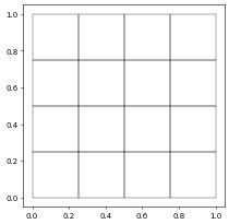
After some general import statements we start our tutorial by setting up a simple Cartesian grid over the domain \(\Omega = [0,1]^2\) subdivided into four intervals in each dimension. We can then show the grid using the plot method - note that direct plotting with MatPlotLib is only supported in 2D, other options for visualization, e.g., using ParaView will be discussed later.

Using the dune.grid.structuredGrid function is the simplest way to construct a grid, more complicated (unstructured) grids can be constructed using a dictionary containing the vertices and the element connectivity or by for example providing a gmsh file. This will be discussed in later section, see for example here for a 3d gmsh file or here for a simple example using a dictionary.

[1]:

from matplotlib import pyplot as plt
import numpy as np

from dune.grid import structuredGrid as leafGridView
gridView = leafGridView([0, 0], [1, 1], [4, 4])
gridView.plot()

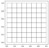
Often the initial grid is a bit coarse - it is very easy to refine it globally.

Note

A grid view object provides read-only access to the entities of all codimensions of a subset of the hierarchical grid. In the following this is called gridView and sometimes simply grid. See [BBD+21], Section 3.1.1, for more details.

Tip

The functions constructing a grid generally return a leaf grid view, i.e., only contains of a view of the finest grid elements. We also provide some special grid views to for example simulate on evolving domains or to simplify efficient local grid adaptivity.

Since a gridView can not be changed directly we need to access the underlying hierarchicalGrid to perform e.g. grid refinement. So to globally refine the grid call

[2]:

gridView.hierarchicalGrid.globalRefine(1)
gridView.plot()

If level>0 then the grid is refined down by the given level and level<0 leads to global coarsening of the grid by the given number of levels (if possible).

Tip

the effect of this refinement will depend on the underlying grid manager. For Cartesian grid for example refining by one level leads a reduction of the grid spacing by 2 while for a bisection grid in \(d\) space dimensions one needs to refine by \(2^{d-1}\) levels to achieve the same effect.

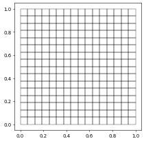
In addition to the globalRefine method on the hierarchicalGrid dune-fem also provides a globalRefine function, which takes the level as the first argument and a hierarchical grid as second argument. This method can also be used to prolong and restrict discrete functions as will be discussed in a later section.

[3]:

from dune.fem import globalRefine
globalRefine(1,gridView.hierarchicalGrid)  # the first argument is the number of refinements to perform
gridView.plot()
globalRefine(-1,gridView.hierarchicalGrid) # coarsen again by one level
gridView.plot()

Grid Functions

Note

A grid function is a function that is defined over a given grid view and is evaluated by using an element of this view and local coordinate within that element, e.g., a quadrature point.

For example:

value = gridFunction(element,localCoordinate)

Alternatively one can obtain a LocalFunction from a grid function which can be bound to an element and then evaluate via local coordinate:

localFunction = gridFunction.localFunction()
for e in grid.elements:
    localFunction.bind(e)
    value = localFunction(x)
    localFunction.unbind()

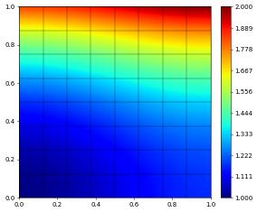
There are multiple ways to construct grid functions. The easiest way it to use UFL expression. Many methods expecting grid functions as argument can also directly handle UFL expression. We can for example integrate a UFL expression over the grid:

[4]:

from ufl import SpatialCoordinate, triangle
x = SpatialCoordinate(triangle)

exact = 1/2*(x[0]**2+x[1]**2) - 1/3*(x[0]**3 - x[1]**3) + 1

from dune.fem import integrate
print( integrate(exact, gridView=gridView, order=5) )

1.3333333333333324

and plot them using matplotlib or write a vtk file for postprocessing

[5]:

from dune.fem.plotting import plotPointData as plot
plot(exact, gridView=gridView)
gridView.writeVTK('exact', pointdata={'exact': exact})

In some cases it can be necessary to convert a UFL expression into a grid function explicitly - for example to be able to evaluate it over each element in the grid (in a later section we provide more detail on how to access the grid interface).

Note

dune.fem.function.gridFunction provides different options for constructing grid functions: it can be used as decorator of Python function, provided with a C++ code snippet, or an ufl expression.

We will discuss the second usages later and have some example for using C++ code snippets in a later section. If the first argument expr is a ufl expression then a grid function is generated which can be efficiently evaluated on both the Python and the C++ side.

Tip

Especially in time critical parts of the code the usage of gridFunction is strongly encouraged to speed up simulations.

Like assemble and integrate, gridFunction takes two additional arguments order and gridView. These are required arguments if a code snippet is used or the gridView is used as a decorator. If the basis of the grid function is a ufl expression these can be omitted in many cases where they can be determined from the expression itself. See the introduction for more detail.

In the next example the gridView argument is required:

[6]:

from dune.fem.function import gridFunction
exact_gf = gridFunction(exact, gridView, name="ufl")
mass = 0
for element in gridView.elements:
    mass += exact_gf(element,[0.5,0.5]) * element.geometry.volume
print(mass)

1.33203125

Another way to obtain a grid function is to use the gridFunction as decorator. This can be obtained from dune.grid but then without UFL support. Using the decorator from dune.fem.function the resulting grid function can be used seamlessly within UFL expressions:

[7]:

from dune.fem.function import gridFunction
@gridFunction(gridView,name="callback",order=1)
def exactLocal(element,xLocal):
    x = element.geometry.toGlobal(xLocal)
    return 1/2.*(x[0]**2+x[1]**2) - 1/3*(x[0]**3 - x[1]**3) + 1

We can use the same approach but with a function using global coordinates but can then be used like any other grid function:

[8]:

@gridFunction(gridView,name="callback",order=1)
def exactGlobal(x):
    return 1/2.*(x[0]**2+x[1]**2) - 1/3*(x[0]**3 - x[1]**3) + 1

lf = exactGlobal.localFunction()

mass = 0
for element in gridView.elements:
    lf.bind(element)
    mass += lf([0.5,0.5]) * element.geometry.volume
    lf.unbind()
print(mass)

1.33203125

As pointed out the dune.fem grid function can be used like any other UFL coefficient to form UFL expressions:

[9]:

print( integrate(abs(exact-exactLocal)) )
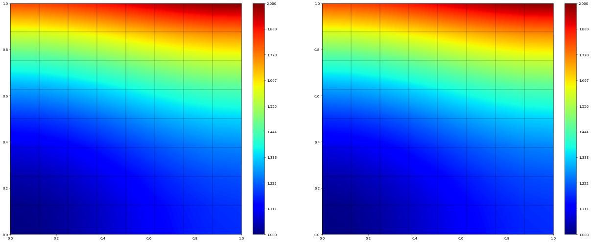
gf = gridFunction(exact-exactLocal+exactGlobal, name="ufl")
fig = plt.figure(figsize=(25,10))
gf.plot(figure=(fig,121))
exactGlobal.plot(figure=(fig,122))

0.0

Converting UFL expressions to grid functions leads to JIT code generation and is therefore efficient when used in other C++ algorithm (like integrate). But more complex control structures are hard to express within UFL. On the other hand using the gridFunction decorator leads to a callback into Python for each evaluation and is therefore much less efficient. An alternative approach is based on writing small C++ snippets implementing the grid function as described in the section on generating C++ Based Grid Functions.

Discrete Spaces

The grid functions set up so far did not involve any discretization, they are exactly evaluated at the given point. We next discuss functions over finite dimensional (discrete) spaces.

Note

A discrete (function) space is a finite dimensional function space defined over a given grid view. Typically these are Finite Element spaces.

Let us start with a Lagrange finite element space consisting of piecewise quadratic functions (order=2):

[10]:

from dune.fem.space import lagrange as solutionSpace
space = solutionSpace(gridView, order=2)

A list of available spaces is shown at the bottom of this page. The main method on the space is interpolate that returns an element of the space (a discrete function) applying the natural interpolation into the space to a given (ufl) expression. This is explained in detail in the next section.

Tip

In addition to the order argument most spaces take an additional dimRange argument to construct vector valued spaces \(V^n\). Note that by default a scalar space is constructed which differs in usage from the space with dimRange=1. Discrete function over the latter have to be treated as vector valued functions of dimension one, e.g., instead of uh*uh one needs uh[0]*uh[0] or ufl.dot(uh,uh).

Two other methods on the discrete spaces worth noting provide access to the local to global dof mapper and evaluate the basis functions.

First we have the mapper method. This returns a callable object which for a given element in the grid, returns the vector of global indices for the basis functions with support on the element:

[11]:

mapper = space.mapper
for i,element in enumerate(gridView.elements):
    print( mapper(element) )
    if i == 4: break # only show indices for first few elements

[0, 81, 1, 153, 225, 154, 9, 89, 10]
[1, 82, 2, 154, 226, 155, 10, 90, 11]
[2, 83, 3, 155, 227, 156, 11, 91, 12]
[3, 84, 4, 156, 228, 157, 12, 92, 13]
[4, 85, 5, 157, 229, 158, 13, 93, 14]

To access the basis functions with support on an element we provide the method evaluateBasis, jacobianBasis:

[12]:

localPoint = [0.1,0.1] # this is in the reference element
for i,element in enumerate(gridView.elements):
    print( space.evaluateBasis(element, localPoint) )
    if i == 4: break
print("convert to a numpy array:", np.array( space.jacobianBasis(element, localPoint) ) )

[Dune::FieldVector<1>(0.518400), Dune::FieldVector<1>(0.259200), Dune::FieldVector<1>(-0.057600), Dune::FieldVector<1>(0.259200), Dune::FieldVector<1>(0.129600), Dune::FieldVector<1>(-0.028800), Dune::FieldVector<1>(-0.057600), Dune::FieldVector<1>(-0.028800), Dune::FieldVector<1>(0.006400)]
[Dune::FieldVector<1>(0.518400), Dune::FieldVector<1>(0.259200), Dune::FieldVector<1>(-0.057600), Dune::FieldVector<1>(0.259200), Dune::FieldVector<1>(0.129600), Dune::FieldVector<1>(-0.028800), Dune::FieldVector<1>(-0.057600), Dune::FieldVector<1>(-0.028800), Dune::FieldVector<1>(0.006400)]
[Dune::FieldVector<1>(0.518400), Dune::FieldVector<1>(0.259200), Dune::FieldVector<1>(-0.057600), Dune::FieldVector<1>(0.259200), Dune::FieldVector<1>(0.129600), Dune::FieldVector<1>(-0.028800), Dune::FieldVector<1>(-0.057600), Dune::FieldVector<1>(-0.028800), Dune::FieldVector<1>(0.006400)]
[Dune::FieldVector<1>(0.518400), Dune::FieldVector<1>(0.259200), Dune::FieldVector<1>(-0.057600), Dune::FieldVector<1>(0.259200), Dune::FieldVector<1>(0.129600), Dune::FieldVector<1>(-0.028800), Dune::FieldVector<1>(-0.057600), Dune::FieldVector<1>(-0.028800), Dune::FieldVector<1>(0.006400)]
[Dune::FieldVector<1>(0.518400), Dune::FieldVector<1>(0.259200), Dune::FieldVector<1>(-0.057600), Dune::FieldVector<1>(0.259200), Dune::FieldVector<1>(0.129600), Dune::FieldVector<1>(-0.028800), Dune::FieldVector<1>(-0.057600), Dune::FieldVector<1>(-0.028800), Dune::FieldVector<1>(0.006400)]
convert to a numpy array: [[[-14.976 -14.976]]

 [[ 18.432  -7.488]]

 [[ -3.456   1.664]]

 [[ -7.488  18.432]]

 [[  9.216   9.216]]

 [[ -1.728  -2.048]]

 [[  1.664  -3.456]]

 [[ -2.048  -1.728]]

 [[  0.384   0.384]]]

Discrete Functions

Note

A special type of grid function is a discrete function living in a discrete (finite dimensional) space. The main property of a discrete function is that it contains a dof vector. In a later section we will see how to extract the underlying dof vector in the form of a numpy or a petsc vector.

The easiest way to construct a discrete function is to use the interpolate method on the discrete function space to create an initialized discrete function or function to create an uninitialized discrete function.

[13]:

# initialized
u_h = space.interpolate(exact, name='u_h')

# uninitialized
u_h = space.function(name='u_h')

On an existing discrete function the interpolate method can be used to reinitialize it

[14]:

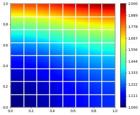
u_h.interpolate( lambda x: 1/2.*(x[0]**2+x[1]**2) - 1/3*(x[0]**3 - x[1]**3) + 1 )
u_h.plot()

Note that in the last example the Python lambda is used as a callback automatically using the same concept used in the gridFunction decorator. As pointed out above there are some methods where these conversions are implicit and no explicit generation of a grid function has to be carried out.

If a discrete function is already available it is possible to call copy to obtain further discrete functions:

[15]:

u_h_n = u_h.copy(name="previous")

Finally, clear can be called on a discrete function which sets all coefficient to zero and assign can be used to copy all coefficients between two discrete function over the same space:

[16]:

u_h_n.clear()
u_h_n.assign( u_h )

All the things we did above with grid functions can be done with discrete functions, e.g., evaluate locally

[17]:

localUh = u_h.localFunction()
mass = 0
for element in gridView.elements:
    localUh.bind(element) # using u_h(element,[0.5,0.5]) also works
    mass += localUh([0.5,0.5]) * element.geometry.volume
    localUh.unbind()
print(mass)

1.33203125

or plot using matplotlib and write a vtk file for postprocessing (using binary data format to reduce size)

[18]:

u_h.plot(gridLines="white", linewidth=2)
from dune.grid import OutputType
gridView.writeVTK('uh', pointdata=[u_h])

Tip

The discrete function u_h already has a name attribute given in the interpolate call. This is used by default in the vtk file. An alternative name can be given by using a dictionary as shown previously.

Of course a discrete function can also be used as a coefficient in a UFL expression

[19]:

print( integrate(abs(exact-u_h)) )

3.1323256792013636e-05

The main difference between a grid function and a discrete function is that the latter has a dofVector attached to it. We can iterate over that easily

[20]:

for d in u_h.dofVector:
    print(d,end=", ")
print()

1.0, 1.0071614583333333, 1.0260416666666667, 1.052734375, 1.0833333333333333, 1.1139322916666667, 1.140625, 1.1595052083333333, 1.1666666666666667, 1.0084635416666667, 1.015625, 1.0345052083333333, 1.0611979166666667, 1.091796875, 1.1223958333333333, 1.1490885416666667, 1.16796875, 1.1751302083333335, 1.0364583333333333, 1.0436197916666667, 1.0625, 1.0891927083333333, 1.1197916666666667, 1.150390625, 1.1770833333333333, 1.1959635416666667, 1.203125, 1.087890625, 1.0950520833333333, 1.1139322916666667, 1.140625, 1.1712239583333333, 1.2018229166666667, 1.228515625, 1.2473958333333333, 1.2545572916666667, 1.1666666666666667, 1.173828125, 1.1927083333333333, 1.2194010416666667, 1.25, 1.2805989583333333, 1.3072916666666667, 1.326171875, 1.3333333333333335, 1.2766927083333333, 1.2838541666666665, 1.302734375, 1.3294270833333333, 1.3600260416666667, 1.390625, 1.4173177083333333, 1.4361979166666667, 1.443359375, 1.421875, 1.4290364583333333, 1.4479166666666665, 1.474609375, 1.5052083333333335, 1.5358072916666665, 1.5625, 1.5813802083333335, 1.5885416666666667, 1.6061197916666665, 1.61328125, 1.6321614583333333, 1.6588541666666665, 1.689453125, 1.7200520833333333, 1.7467447916666665, 1.765625, 1.7727864583333335, 1.8333333333333333, 1.8404947916666665, 1.859375, 1.8860677083333333, 1.9166666666666665, 1.947265625, 1.9739583333333333, 1.9928385416666665, 2.0, 1.0018717447916667, 1.015380859375, 1.0386555989583333, 1.0677897135416667, 1.098876953125, 1.1280110677083333, 1.1512858072916667, 1.164794921875, 1.0103352864583333, 1.0238444010416667, 1.047119140625, 1.0762532552083333, 1.1073404947916667, 1.136474609375, 1.1597493489583333, 1.1732584635416667, 1.038330078125, 1.0518391927083333, 1.0751139322916667, 1.104248046875, 1.1353352864583333, 1.1644694010416667, 1.187744140625, 1.2012532552083335, 1.0897623697916667, 1.103271484375, 1.1265462239583333, 1.1556803385416667, 1.186767578125, 1.2159016927083333, 1.2391764322916667, 1.252685546875, 1.1685384114583333, 1.1820475260416667, 1.205322265625, 1.2344563802083333, 1.2655436197916667, 1.294677734375, 1.3179524739583335, 1.3314615885416667, 1.278564453125, 1.2920735677083333, 1.3153483072916665, 1.344482421875, 1.3755696614583333, 1.4047037760416667, 1.427978515625, 1.4414876302083335, 1.4237467447916665, 1.437255859375, 1.4605305989583333, 1.4896647135416665, 1.520751953125, 1.5498860677083335, 1.5731608072916665, 1.586669921875, 1.6079915364583333, 1.6215006510416665, 1.644775390625, 1.6739095052083333, 1.7049967447916665, 1.734130859375, 1.7574055989583335, 1.7709147135416665, 1.835205078125, 1.8487141927083333, 1.8719889322916665, 1.901123046875, 1.9322102864583333, 1.9613444010416665, 1.984619140625, 1.9981282552083335, 1.0020345052083333, 1.0091959635416667, 1.028076171875, 1.0547688802083333, 1.0853678385416667, 1.115966796875, 1.1426595052083333, 1.1615397135416667, 1.168701171875, 1.019775390625, 1.0269368489583333, 1.0458170572916667, 1.072509765625, 1.1031087239583333, 1.1337076822916667, 1.160400390625, 1.1792805989583333, 1.1864420572916667, 1.0590006510416667, 1.066162109375, 1.0850423177083333, 1.1117350260416667, 1.142333984375, 1.1729329427083333, 1.1996256510416667, 1.218505859375, 1.2256673177083335, 1.1236165364583333, 1.1307779947916667, 1.149658203125, 1.1763509114583333, 1.2069498697916667, 1.237548828125, 1.2642415364583335, 1.2831217447916667, 1.290283203125, 1.217529296875, 1.2246907552083333, 1.2435709635416667, 1.270263671875, 1.3008626302083333, 1.3314615885416667, 1.358154296875, 1.3770345052083335, 1.3841959635416667, 1.3446451822916665, 1.351806640625, 1.3706868489583333, 1.3973795572916665, 1.427978515625, 1.4585774739583333, 1.4852701822916667, 1.504150390625, 1.5113118489583335, 1.5088704427083333, 1.5160319010416665, 1.534912109375, 1.5616048177083333, 1.5922037760416665, 1.622802734375, 1.6494954427083335, 1.6683756510416665, 1.675537109375, 1.714111328125, 1.7212727864583333, 1.7401529947916665, 1.766845703125, 1.7974446614583333, 1.8280436197916665, 1.854736328125, 1.8736165364583335, 1.8807779947916665, 1.00390625, 1.0174153645833333, 1.0406901041666667, 1.06982421875, 1.1009114583333333, 1.1300455729166667, 1.1533203125, 1.1668294270833335, 1.0216471354166667, 1.03515625, 1.0584309895833333, 1.0875651041666667, 1.11865234375, 1.1477864583333333, 1.1710611979166667, 1.1845703125, 1.0608723958333333, 1.0743815104166667, 1.09765625, 1.1267903645833333, 1.1578776041666667, 1.18701171875, 1.2102864583333333, 1.2237955729166667, 1.12548828125, 1.1389973958333333, 1.1622721354166667, 1.19140625, 1.2224934895833333, 1.2516276041666667, 1.27490234375, 1.2884114583333335, 1.2194010416666667, 1.23291015625, 1.2561848958333333, 1.2853190104166667, 1.31640625, 1.3455403645833333, 1.3688151041666667, 1.38232421875, 1.3465169270833333, 1.3600260416666665, 1.38330078125, 1.4124348958333333, 1.4435221354166667, 1.47265625, 1.4959309895833335, 1.5094401041666667, 1.5107421875, 1.5242513020833333, 1.5475260416666665, 1.57666015625, 1.6077473958333335, 1.6368815104166665, 1.66015625, 1.6736653645833335, 1.7159830729166665, 1.7294921875, 1.7527669270833333, 1.7819010416666665, 1.81298828125, 1.8421223958333333, 1.8653971354166665, 1.87890625,

In addition to clear and assign we can also add (scalar multiples of) discrete functions together or multiply them by a scalar which will directly change the underlying dofVector - this can only be done in place, so u_h *= 2 changes the dof vector while u_h*2 results in an UFL expression. Here are some examples:

[21]:

u_h_n *= 2
u_h   += u_h_n
# this is equivalent to
u_h.axpy(2,u_h_n)

We started with u_h_n=u_h so after these changes each dof in u_h should be seven times its original value

[22]:

for d in u_h.dofVector:
    print(d,end=", ")
print()

7.0, 7.050130208333333, 7.182291666666667, 7.369140625, 7.583333333333333, 7.797526041666667, 7.984375, 8.116536458333332, 8.166666666666668, 7.059244791666667, 7.109375, 7.241536458333333, 7.428385416666667, 7.642578125, 7.856770833333333, 8.043619791666668, 8.17578125, 8.225911458333334, 7.255208333333333, 7.305338541666667, 7.4375, 7.624348958333333, 7.838541666666667, 8.052734375, 8.239583333333332, 8.371744791666668, 8.421875, 7.615234375, 7.665364583333333, 7.797526041666667, 7.984375, 8.198567708333332, 8.412760416666668, 8.599609375, 8.731770833333332, 8.781901041666668, 8.166666666666668, 8.216796875, 8.348958333333332, 8.535807291666668, 8.75, 8.964192708333332, 9.151041666666668, 9.283203125, 9.333333333333334, 8.936848958333332, 8.986979166666666, 9.119140625, 9.305989583333332, 9.520182291666668, 9.734375, 9.921223958333332, 10.053385416666668, 10.103515625, 9.953125, 10.003255208333332, 10.135416666666666, 10.322265625, 10.536458333333334, 10.750651041666666, 10.9375, 11.069661458333334, 11.119791666666668, 11.242838541666666, 11.29296875, 11.425130208333332, 11.611979166666666, 11.826171875, 12.040364583333332, 12.227213541666666, 12.359375, 12.409505208333334, 12.833333333333332, 12.883463541666666, 13.015625, 13.202473958333332, 13.416666666666666, 13.630859375, 13.817708333333332, 13.949869791666666, 14.0, 7.013102213541667, 7.107666015625, 7.270589192708333, 7.474527994791667, 7.692138671875, 7.896077473958333, 8.059000651041668, 8.153564453125, 7.072347005208333, 7.166910807291667, 7.329833984375, 7.533772786458333, 7.751383463541667, 7.955322265625, 8.118245442708332, 8.212809244791668, 7.268310546875, 7.362874348958333, 7.525797526041667, 7.729736328125, 7.947347005208333, 8.151285807291668, 8.314208984375, 8.408772786458334, 7.628336588541667, 7.722900390625, 7.885823567708333, 8.089762369791668, 8.307373046875, 8.511311848958332, 8.674235026041668, 8.768798828125, 8.179768880208332, 8.274332682291668, 8.437255859375, 8.641194661458332, 8.858805338541668, 9.062744140625, 9.225667317708334, 9.320231119791668, 8.949951171875, 9.044514973958332, 9.207438151041666, 9.411376953125, 9.628987630208332, 9.832926432291668, 9.995849609375, 10.090413411458334, 9.966227213541666, 10.060791015625, 10.223714192708332, 10.427652994791666, 10.645263671875, 10.849202473958334, 11.012125651041666, 11.106689453125, 11.255940755208332, 11.350504557291666, 11.513427734375, 11.717366536458332, 11.934977213541666, 12.138916015625, 12.301839192708334, 12.396402994791666, 12.846435546875, 12.940999348958332, 13.103922526041666, 13.307861328125, 13.525472005208332, 13.729410807291666, 13.892333984375, 13.986897786458334, 7.014241536458333, 7.064371744791667, 7.196533203125, 7.383382161458333, 7.597574869791667, 7.811767578125, 7.998616536458333, 8.130777994791668, 8.180908203125, 7.138427734375, 7.188557942708333, 7.320719401041667, 7.507568359375, 7.721761067708333, 7.935953776041667, 8.122802734375, 8.254964192708332, 8.305094401041668, 7.413004557291667, 7.463134765625, 7.595296223958333, 7.782145182291667, 7.996337890625, 8.210530598958332, 8.397379557291668, 8.529541015625, 8.579671223958334, 7.865315755208333, 7.915445963541667, 8.047607421875, 8.234456380208332, 8.448649088541668, 8.662841796875, 8.849690755208334, 8.981852213541668, 9.031982421875, 8.522705078125, 8.572835286458332, 8.704996744791668, 8.891845703125, 9.106038411458332, 9.320231119791668, 9.507080078125, 9.639241536458334, 9.689371744791668, 9.412516276041666, 9.462646484375, 9.594807942708332, 9.781656901041666, 9.995849609375, 10.210042317708332, 10.396891276041668, 10.529052734375, 10.579182942708334, 10.562093098958332, 10.612223307291666, 10.744384765625, 10.931233723958332, 11.145426432291666, 11.359619140625, 11.546468098958334, 11.678629557291666, 11.728759765625, 11.998779296875, 12.048909505208332, 12.181070963541666, 12.367919921875, 12.582112630208332, 12.796305338541666, 12.983154296875, 13.115315755208334, 13.165445963541666, 7.02734375, 7.121907552083333, 7.284830729166667, 7.48876953125, 7.706380208333333, 7.910319010416667, 8.0732421875, 8.167805989583334, 7.151529947916667, 7.24609375, 7.409016927083333, 7.612955729166667, 7.83056640625, 8.034505208333332, 8.197428385416668, 8.2919921875, 7.426106770833333, 7.520670572916667, 7.68359375, 7.887532552083333, 8.105143229166668, 8.30908203125, 8.472005208333332, 8.566569010416668, 7.87841796875, 7.972981770833333, 8.135904947916668, 8.33984375, 8.557454427083332, 8.761393229166668, 8.92431640625, 9.018880208333334, 8.535807291666668, 8.63037109375, 8.793294270833332, 8.997233072916668, 9.21484375, 9.418782552083332, 9.581705729166668, 9.67626953125, 9.425618489583332, 9.520182291666666, 9.68310546875, 9.887044270833332, 10.104654947916668, 10.30859375, 10.471516927083334, 10.566080729166668, 10.5751953125, 10.669759114583332, 10.832682291666666, 11.03662109375, 11.254231770833334, 11.458170572916666, 11.62109375, 11.715657552083334, 12.011881510416666, 12.1064453125, 12.269368489583332, 12.473307291666666, 12.69091796875, 12.894856770833332, 13.057779947916666, 13.15234375,

Operators and Schemes

In the previous section we have already seen how to assemble system matrices for linear PDEs and how to construct schemes for non-linear problems. We also discussed that we can directly use grid functions and dune.ufl.Constant instances within UFL expressions and forms - in the final example of this section we will give an example for this in the context of a time dependent problems.

Tip

The main advantage of using dune.ufl.Constant and grid functions is to be able to change details in a form without requiring any recompilation of the model. An example would be in a time dependent problem a time varying coefficient or changing the time step adaptively during the simulation.

Let us first consider a simple linear elliptic problem

\[-\triangle u + \alpha u = f\]

with Dirichlet and Neuman boundary data given by \(g_D,g_N\) and where \(\alpha\) is a real valued parameter. We choose \(f,g_N,g_D\) so that the exact solution for \(\alpha=0\) is given by \begin{align*} u(x) = \left(\frac{1}{2}(x^2 + y^2) - \frac{1}{3}(x^3 - y^3)\right) + 1 \end{align*} which is the grid function exact we have already defined above.

Note

The class dune.ufl.DirichletBC is used to fix Dirichlet conditions \(u=g\) on \(\Gamma\subset\partial\Omega\). It constructor takes three arguments: the discrete space for \(u\), the data \(g\), and a description of \(\Gamma\). Multiple instances can be used to fix Dirichlet conditions on different parts of the boundary as described in the Section on general boundary conditions.

To assemble a system matrix from a ufl form one can either use dune.fem.assemble which is especially useful for simple linear models as discussed in the previous section. For more control one should use schemes or operators:

Note

A scheme implements a Galerkin scheme for a given weak form for a wide range of PDEs, where the model (integrands) is provided as ufl form. Mathematically a scheme implements an operator \(L\colon V_h\to V_h\) with equal (discrete) domain and range space. The scheme provides a solve method which computes \(u=L^{-1}(g)\) for given \(g\). By default a root of \(L\) is computed but a right hand side \(g\) can be provided to solve \(L[u_h]=g\).

Note

The more general case is covered by classes in dune.fem.operator for operators \(L\colon V_h\to W_h\) with different domain and range spaces. See here for more details on the concepts and a summary of the API for operators and schemes.

[23]:

from ufl import (TestFunction, TrialFunction, SpatialCoordinate, FacetNormal,
                 dx, ds, grad, div, inner, dot, sin, cos, pi, conditional)
from dune.ufl import Constant, DirichletBC
from dune.fem.scheme import galerkin as solutionScheme

alpha = Constant(1,name="mass")   # start with alpha=1
x     = SpatialCoordinate(space)
u     = TrialFunction(space)
v     = TestFunction(space)
f     = -div( grad(exact) )
g_N   = grad(exact)
n     = FacetNormal(space)
b     = f*v*dx + dot(g_N,n)*conditional(x[0]>=1e-8,1,0)*v*ds
a     = dot(grad(u), grad(v)) * dx + alpha*u*v * dx
dbc   = DirichletBC(space,exact,x[0]<=1e-8)

scheme = solutionScheme([a == b, dbc], solver='cg')
scheme.solve(target = u_h)

h1error = dot(grad(u_h - exact), grad(u_h - exact))
error = np.sqrt(integrate(h1error))
print("Number of elements:",gridView.size(0),
      "number of dofs:",space.size,"H^1 error:", error)

Number of elements: 64 number of dofs: 289 H^1 error: 0.5635700799029998

Note

The dune.ufl.Constant class implements a scalar or vector valued constant with a name. This constant can be used within a ufl form and after the ufl form was converted into a scheme or operator the given name can be used to change the constant within the form efficiently, e.g., we can adapt the point in time or time step during the simulation without requiring any additional just in time compilation.

Instances of dune.ufl.Constant have an attribute value to read and change the constant. Setting the value, will change it everywhere it is used. In addition a scheme/operator provides the attribute model which has an attribute name for each constant with name name contained in the ufl form used to construct the scheme/operator. Cchanging the value of the constants through the model attribute only changes it within that model and not globally.

[24]:

print(scheme.model.mass, alpha.value)
scheme.model.mass = 2
print(scheme.model.mass, alpha.value)
alpha.value = 0
print(scheme.model.mass, alpha.value)

1.0 1.0
2.0 1.0
0.0 0.0

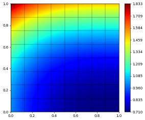
Note that now \(\alpha=0\) so we have the correct exact solution and can compute the errors:

[25]:

scheme.solve(target = u_h)

h1error = dot(grad(u_h - exact), grad(u_h - exact))
error = np.sqrt(integrate(h1error))
print("Number of elements:",gridView.size(0),
      "number of dofs:",space.size,"H^1 error:", error)
u_h.plot()

Number of elements: 64 number of dofs: 289 H^1 error: 0.0016470196146885557

Or switch to \(\alpha=1\) to directly solve a different PDE without needing to recompile anything:

[26]:

alpha.value = 1
scheme.solve(target = u_h)
u_h.plot()

Tip

Changing the values of constants using the value attribute on dune.ufl.Constant is generally the option with the least chance for surprise. The scheme.model.name approach is useful if the instance of dune.ufl.Constant is not available anymore, e.g., a scheme was returned by some function which constructed the constants as local variables.

A Nonlinear Time Dependent Problem

As a final example in this section we will study the Forchheimer problem [Kie15] which is a scalar, nonlinear parabolic equation \begin{equation} \partial_tu - \nabla\cdot K(\nabla u)\nabla u = f \end{equation} where the diffusion tensor is given by \begin{equation} K(\nabla u) = \frac{2}{1+\sqrt{1+4|\nabla u|}} \end{equation} and \(f=f(x,t)\) is some time dependent forcing term. On the boundary we prescribe Neumann boundary and initial conditions \(u=u_0\).

We will solve this problem in variational form and using the Crank Nicolson method for the time discretization

\begin{equation} \begin{split} \int_{\Omega} \frac{u^{n+1}-u^n}{\Delta t} \varphi + \frac{1}{2}K(\nabla u^{n+1}) \nabla u^{n+1} \cdot \nabla \varphi \ + \frac{1}{2}K(\nabla u^n) \nabla u^n \cdot \nabla \varphi v\ dx \\ - \int_{\Omega} \frac{1}{2}(f(x,t^n)+f(x,t^n+\Delta t) \varphi\ dx - \int_{\partial \Omega} \frac{1}{2}(g(x,t^n)+g(x,t^n+\Delta t)) v\ ds = 0. \end{split} \end{equation}

on a domain \(\Omega=[0,1]^2\). We choose \(f,g\) so that the exact solution is given by \begin{align*} u(x,t) = e^{-2t}\left(\frac{1}{2}(x^2 + y^2) - \frac{1}{3}(x^3 - y^3)\right) + 1 \end{align*} We solve this problem using a quadratic finite element space. We first setup this space, define the initial data, and a second discrete function to store the solution at the current time step (u_h will be used to store the next time step):

[27]:

space = solutionSpace(gridView, order=2)
u_h   = space.interpolate(0, name='u_h')
u_h_n = u_h.copy(name="previous")

x = SpatialCoordinate(space)
initial = 1/2*(x[0]**2+x[1]**2) - 1/3*(x[0]**3 - x[1]**3) + 1

Next we setup the form \(a=a(u,v)\) which depends on time \(t\) and the chosen time step \(\Delta t\). Since we want to be able to change these during the simulation (we need to do this for \(t\) and might want to do this for \(\Delta t\) we use the dune.ufl.Constant which stores a mutable scalar and can be used within a ufl expression:

[28]:

from dune.fem.scheme import galerkin as solutionScheme
from ufl import FacetNormal, ds, dx, inner, dot, div, grad, sqrt, exp, TrialFunction, TestFunction
from dune.ufl import Constant
dt = Constant(0, name="dt")    # time step
t  = Constant(0, name="t")     # current time
u = TrialFunction(space)
v = TestFunction(space)

abs_du = lambda u: sqrt(inner(grad(u), grad(u)))
K = lambda u: 2/(1 + sqrt(1 + 4*abs_du(u)))
a = ( dot((u - u_h_n)/dt, v) \
    + 0.5*dot(K(u)*grad(u), grad(v)) \
    + 0.5*dot(K(u_h_n)*grad(u_h_n), grad(v)) ) * dx

To define the right hand side we use the given function \(u\) to define the forcing \(f\) and the boundary flux \(g\)

[29]:

exact = lambda t: exp(-2*t)*(initial - 1) + 1
f     = lambda s: -2*exp(-2*s)*(initial - 1) - div( K(exact(s))*grad(exact(s)) )
g = lambda s: K(exact(s))*grad(exact(s))
n = FacetNormal(space)
b = 0.5*(f(t)+f(t+dt))*v*dx + 0.5*dot(g(t)+g(t+dt),n)*v*ds

With the model described as a ufl form, we can again construct a scheme class that provides the solve method which we can use to evolve the solution from one time step to the next. As already mentioned the solve methods always assumes that the problem is non-linear and use a Newton method to solve the problem:

[30]:

scheme = solutionScheme(a == b, solver='cg')

Optionally, we may want to increase the default quadrature orders which are 2 * space.order for element integrals and 2 * space.order + 1 for surface integrals. Depending on the data this might not be enough. Then we simply set the integration orders by hand like in the following example, by calling the method setQuadratureOrders(interiorOrder, surfaceOrder).

[31]:

#scheme.setQuadratureOrders( 2*space.order, 2*space.order+1 )

Since we have forced the system towards a given solution, we can compute the discretization error. First we define ufl expressions for the \(L^2\) and \(H^1\) norms and will use those to compute the experimental order of convergence of the scheme by computing the time evolution on different grid levels. We use dune.fem.function.gridFunction to generate code for the errors which can be more efficient than using the ufl expressions directly.

[32]:

endTime    = 0.25
exact_end  = exact(endTime)
l2error = gridFunction(dot(u_h - exact_end, u_h - exact_end), name="l2error")
h1error = gridFunction(dot(grad(u_h - exact_end), grad(u_h - exact_end)), name="h1error")

Now we evolve the solution from time \(t=0\) to \(t=T\) in a loop. Since the PDE model has time dependent coefficient (through the forcing term), we need to update the t constant used to define the model before each step. A second constant we used to define the model was dt which defines the time step. We keep this constant and set it to \(0.002\) at the beginning of the simulation. This value could be changed in each time step:

[33]:

dt.value = 0.01
time = 0
u_h.interpolate(initial)
while time < (endTime - 1e-6):
    t.value = time
    u_h_n.assign(u_h)
    scheme.solve(target=u_h)
    time += dt.value

errors = [np.sqrt(e) for e in integrate([l2error,h1error])]
print('grid size:', gridView.size(0))
print('\t | u_h - u | =', '{:0.5e}'.format(errors[0]))
print('\t | grad(uh - u) | =', '{:0.5e}'.format(errors[1]))
u_h.plot()
gridView.writeVTK('forchheimer', pointdata={'u': u_h, 'l2error': l2error, 'h1error': h1error})

grid size: 64
         | u_h - u | = 1.98216e-05
         | grad(uh - u) | = 9.99185e-04

We can refine the grid once and recompute the solution on the finer grid.

[34]:

globalRefine(1, gridView.hierarchicalGrid)
dt.value /= 2
u_h.interpolate(initial)
time = 0
while time < (endTime - 1e-6):
    t.value = time
    u_h_n.assign(u_h)
    scheme.solve(target=u_h)
    time += dt.value

errorsFine = [np.sqrt(e) for e in integrate([l2error,h1error])]
print('grid size:', gridView.size(0))
print('\t | u_h - u | =', '{:0.5e}'.format(errorsFine[0]))
print('\t | grad(uh - u) | =', '{:0.5e}'.format(errorsFine[1]))
u_h.plot()

grid size: 256
         | u_h - u | = 2.69665e-06
         | grad(uh - u) | = 2.49777e-04

To check that everything is working as expected let’s compute the experimental order of convergence (convergence should be cubic for \(L^2\)-error and quadratic for the \(H^1\)-error:

[35]:

eocs = [ round(np.log(fine/coarse)/np.log(0.5),2)
         for fine,coarse in zip(errorsFine,errors) ]
print("EOCs:",eocs)

EOCs: [2.88, 2.0]

Listing Available Dune Components

The available realization of a given interface, i.e., the available grid implementations, depends on the modules found during configuration. Getting access to all available components is straightforward:

[36]:

from dune.utility import components
# to get a list of all available components:
components()
# to get for example all available grid implementations:
components("grid")

available categories are:
 discretefunction,function,grid,model,operator,scheme,solver,space,view
available entries for this category are:
entry         function          module
----------------------------------------------
agglomerate   polyGrid          dune.vem.vem
alberta       albertaGrid       dune.grid
alu           aluGrid           dune.alugrid
aluconform    aluConformGrid    dune.alugrid
alucube       aluCubeGrid       dune.alugrid
alusimplex    aluSimplexGrid    dune.alugrid
mmesh         mmesh             dune.mmesh
oned          onedGrid          dune.grid
polygon       polygonGrid       dune.polygongrid
sp            spIsotropicGrid   dune.spgrid
spanisotropic spAnisotropicGrid dune.spgrid
spbisection   spBisectionGrid   dune.spgrid
spisotropic   spIsotropicGrid   dune.spgrid
ug            ugGrid            dune.grid
yasp          yaspGrid          dune.grid
----------------------------------------------

Available discrete function spaces are:

[37]:

components("space")

available entries for this category are:
entry             function          module
------------------------------------------------
bbdg              bbdgSpace         dune.vem.vem
bdm               bdm               dune.fem.space
combined          combined          dune.fem.space
composite         composite         dune.fem.space
dglagrange        dglagrange        dune.fem.space
dglagrangelobatto dglagrangelobatto dune.fem.space
dglegendre        dglegendre        dune.fem.space
dglegendrehp      dglegendrehp      dune.fem.space
dgonb             dgonb             dune.fem.space
dgonbhp           dgonbhp           dune.fem.space
finitevolume      finiteVolume      dune.fem.space
lagrange          lagrange          dune.fem.space
lagrangehp        lagrangehp        dune.fem.space
p1bubble          p1Bubble          dune.fem.space
product           product           dune.fem.space
rannacherturek    rannacherTurek    dune.fem.space
raviartthomas     raviartThomas     dune.fem.space
vem               vemSpace          dune.vem.vem
------------------------------------------------

Available grid functions are:

[38]:

components("function")

available entries for this category are:
entry        function          module
----------------------------------------------
discrete     discreteFunction  dune.fem.function
gridfunction gridFunction      dune.fem.function
levels       levelFunction     dune.fem.function
partitions   partitionFunction dune.fem.function
----------------------------------------------

Available schemes:

[39]:

components("scheme")

available entries for this category are:
entry      function         module
-----------------------------------------
bbdg       bbdgScheme       dune.vem.vem
dg         dg               dune.fem.scheme
dggalerkin dgGalerkin       dune.fem.scheme
galerkin   galerkin         dune.fem.scheme
h1         h1               dune.fem.scheme
h1galerkin h1Galerkin       dune.fem.scheme
linearized linearized       dune.fem.scheme
rungekutta rungeKuttaSolver dune.femdg
vem        vemScheme        dune.vem.vem
-----------------------------------------

This page was generated from the notebook concepts_nb.ipynb and is part of the tutorial for the dune-fem python bindings