Linear Elasticity: a Deformed Beam

We first setup the domain and solution space, together with the vector valued discrete function \(u\) which describes the displacement field:

from matplotlib import pyplot
from dune.fem.plotting import plotPointData as plot
from dune.grid import structuredGrid as leafGridView
from dune.fem.space import lagrange as solutionSpace
from dune.fem.scheme import galerkin as solutionScheme

from ufl import *
import dune.ufl

gridView = leafGridView([0, 0], [1, 0.15], [100, 15])
space = solutionSpace(gridView, dimRange=2, order=2, storage="istl")
displacement = space.interpolate([0,0], name="displacement")

We want clamped boundary conditions on the left, i.e., zero displacement

x = SpatialCoordinate(space)
dbc = dune.ufl.DirichletBC(space, as_vector([0,0]), x[0]<1e-10)

Next we define the variational problem starting with a few constants describing material properties (\(\mu,\lambda,\rho\)) and the gravitational force

lamb = 0.1     # 1st Lamé coefficient (\lambda)
mu   = 1       # 2nd Lamé coefficient (\mu)
rho  = 1/1000. # material density
g    = 9.8     # gravitational acceleration

Next we define the strain and stress \begin{align*} \epsilon(u) &= \frac{1}{2}(\nabla u + \nabla u^T) \\ \sigma(u) &= 2\mu\epsilon(u) + \lambda\nabla\cdot u I \end{align*} where \(I\) is the identity matrix.

epsilon = lambda u: 0.5*(nabla_grad(u) + nabla_grad(u).T)
sigma = lambda u: lamb*nabla_div(u)*Identity(2) + 2*mu*epsilon(u)

Finally we define the variational problem \begin{align*} \int_\Omega \sigma(u)\colon\epsilon(v) = \int_\Omega (0,-\rho g)\cdot v \end{align*} and solve the system

u = TrialFunction(space)
v = TestFunction(space)
equation = inner(sigma(u), epsilon(v))*dx == dot(as_vector([0,-rho*g]),v)*dx

scheme = solutionScheme([equation, dbc], solver='cg',
            parameters = {"newton.linear.preconditioning.method": "ilu"} )
info = scheme.solve(target=displacement)

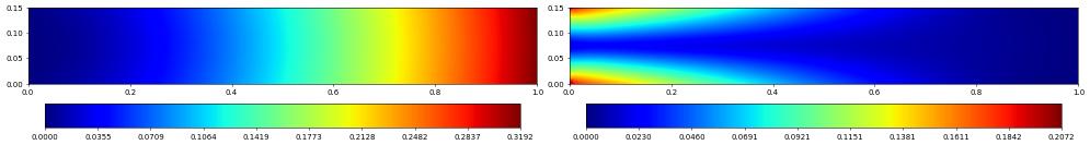
We can directly plot the magnitude of the displacement field and the stress

fig = pyplot.figure(figsize=(20,10))
displacement.plot(gridLines=None, figure=(fig, 121), colorbar="horizontal")
s = sigma(displacement) - (1./3)*tr(sigma(displacement))*Identity(2)
von_Mises = sqrt(3./2*inner(s, s))
plot(von_Mises, grid=gridView, gridLines=None, figure=(fig, 122), colorbar="horizontal")

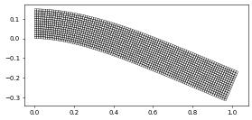
Finally we can plot the actual displaced beam using a grid view that allows us to add a transformation of the geometry of each entity in the grid by prociding a grid function to the constructor. Note that this also allows for higher order transformation like in this case where the transformation is given by a second order Lagrange discrete function. We will highlight the flexibility of the # GeometryGridView in further examples:

from dune.fem.view import geometryGridView
position = space.interpolate( x+displacement, name="position" )
beam = geometryGridView( position )
beam.plot()

This page was generated from the notebook elasticity_nb.ipynb and is part of the tutorial for the dune-fem python bindings