Re-entrant Corner Problem

Here we will consider the classic re-entrant corner problem, \begin{align*} -\Delta u &= f, && \text{in } \Omega, \\ u &= g, && \text{on } \partial\Omega, \end{align*} where the domain is given using polar coordinates, \begin{gather*} \Omega = \{ (r,\varphi)\colon r\in(0,1), \varphi\in(0,\Phi) \}~. \end{gather*} For the boundary condition \(g\), we set it to the trace of the function \(u\), given by \begin{gather*} u(r,\varphi) = r^{\frac{\pi}{\Phi}} \sin\big(\frac{\pi}{\Phi} \varphi \big) \end{gather*}

import numpy
import matplotlib.pyplot as pyplot
from dune.fem.plotting import plotPointData as plot
import dune.grid as grid
import dune.fem as fem
from dune.fem.view import adaptiveLeafGridView as adaptiveGridView
from dune.fem.space import lagrange as solutionSpace
from dune.alugrid import aluConformGrid as leafGridView
from dune.fem.function import gridFunction
from dune.fem import integrate
from ufl import *
from dune.ufl import DirichletBC


# set the angle for the corner (0<angle<=360)
cornerAngle = 320.

# use a second order space
order = 2

We first define the domain and set up the grid and space. We need this twice - once for a computation on a globally refined grid and once for an adaptive one so we put the setup into a function:

We first define the grid for this domain (vertices are the origin and 4 equally spaced points on the unit sphere starting with (1,0) and ending at (cos(cornerAngle), sin(cornerAngle))

Next we define the model together with the exact solution.

def setup():
    vertices = numpy.zeros((8, 2))
    vertices[0] = [0, 0]
    for i in range(0, 7):
        vertices[i+1] = [numpy.cos(cornerAngle/6*numpy.pi/180*i),
                         numpy.sin(cornerAngle/6*numpy.pi/180*i)]
    triangles = numpy.array([[2,1,0], [0,3,2], [4,3,0],
                             [0,5,4], [6,5,0], [0,7,6]])
    domain = {"vertices": vertices, "simplices": triangles}
    gridView = adaptiveGridView( leafGridView(domain) )
    gridView.hierarchicalGrid.globalRefine(2)
    space = solutionSpace(gridView, order=order, storage="numpy")

    from dune.fem.scheme import galerkin as solutionScheme
    u = TrialFunction(space)
    v = TestFunction(space)
    x = SpatialCoordinate(space.cell())

    # exact solution for this angle
    Phi = cornerAngle / 180 * pi
    phi = atan_2(x[1], x[0]) + conditional(x[1] < 0, 2*pi, 0)
    exact = dot(x, x)**(pi/2/Phi) * sin(pi/Phi * phi)
    a = dot(grad(u), grad(v)) * dx

    # set up the scheme
    laplace = solutionScheme([a==0, DirichletBC(space, exact, 1)], solver="cg",
                parameters={"newton.linear.preconditioning.method":"jacobi"})
    uh = space.interpolate([0], name="solution")
    return uh, exact, laplace

We will start with computing the \(H^1\) error on a sequence of globally refined grids

Note that by using fem.globalRefine instead of hierarchicalGrid.globalRefine we can prolongate discrete functions to the next level. The second argument can also be a list/tuple of discrete functions to prolong. With this approach we obtain a good initial guess for solving the problem on the refined grid.

uh, exact, laplace = setup()
h1error = gridFunction(dot(grad(uh - exact), grad(uh - exact)))
errorGlobal = []
dofsGlobal  = []
for count in range(10):
    laplace.solve(target=uh)
    error = numpy.sqrt(integrate(h1error, order=5))
    errorGlobal += [error]
    dofsGlobal  += [uh.space.size]
    print(count, ": size=", uh.space.gridView.size(0), "error=", error)
    fem.globalRefine(1,uh)

0 : size= 32 error= 0.18655122279356964
1 : size= 68 error= 0.16034368267325266
2 : size= 144 error= 0.12554948815618358
3 : size= 296 error= 0.10825248980058133
4 : size= 608 error= 0.08486347007968399
5 : size= 1232 error= 0.07320710422512619
6 : size= 2496 error= 0.05741715963355946
7 : size= 5024 error= 0.04954133581605651
8 : size= 10112 error= 0.038864295305858367
9 : size= 20288 error= 0.03353671438408608

Theory tells us that \begin{align*} \int_\Omega |\nabla(u-u_h)|^2 \leq \sum_K \eta_K, \end{align*} where on each element \(K\) of the grid the local estimator is given by \begin{align*} \eta_K = h_K^2 \int_K |\triangle u_h|^2 + \frac{1}{2}\sum_{S\subset \partial K} h_S \int_S [\nabla u_h]^2. \end{align*} Here \([\cdot]\) is the jump in normal direction over the edges of the grid.

We compute the elementwise indicator by defining a bilinear form \begin{align*} \eta(u,v) = \int_\Omega h^2 |\triangle u_h|^2 v + \int_{I_h} h_S [\nabla u_h]^2 \{v\}, \end{align*} where \(\{\cdot\}\) is the average over the cell edges and \([\cdot]\) the jump. With \(h\) and \(h_S\) we denote local grid spacings and with \(I_h\) the set of all facets in the grid. This bilinear form can be easily written in UFL and by using it to define a discrete operator \(L\) from the second order Lagrange space into a space containing piecewise constant functions we have \(L[u_h]|_{K} = \eta_K\).

uh, exact, laplace = setup()

from dune.fem.space import finiteVolume as estimatorSpace
from dune.fem.operator import galerkin as estimatorOp

fvspace = estimatorSpace(uh.space.gridView)
estimate = fvspace.interpolate([0], name="estimate")

u = TrialFunction(uh.space.as_ufl())
v = TestFunction(fvspace)
hT = MaxCellEdgeLength(fvspace.cell())
he = MaxFacetEdgeLength(fvspace.cell())('+')
n = FacetNormal(fvspace.cell())
estimator_ufl = hT**2 * (div(grad(u)))**2 * v * dx +        he * inner(jump(grad(u)), n('+'))**2 * avg(v) * dS
estimator = estimatorOp(estimator_ufl)
tolerance = 0.05

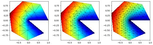
Let us solve over a loop (solve,estimate,mark) and plot the solutions side by side.

h1error = gridFunction(dot(grad(uh - exact), grad(uh - exact)))
fig = pyplot.figure(figsize=(10,10))
count = 0
errorVector    = []
estimateVector = []
dofs           = []
while True:
    laplace.solve(target=uh)
    if count%9 == 8:
        plot(uh, figure=(fig, 131+count//9), colorbar=False)
    error = numpy.sqrt(integrate(h1error, order=5))
    estimator(uh, estimate)
    eta = numpy.sqrt( sum(estimate.dofVector) )
    dofs           += [uh.space.size]
    errorVector    += [error]
    estimateVector += [eta]
    if count%3 == 2:
        print(count, ": size=", uh.space.gridView.size(0), "estimate=", eta, "error=", error)
    if eta < tolerance:
        break
    marked = fem.doerflerMark(estimate,0.6,layered=0.1)
    fem.adapt(uh) # can also be a list or tuple of function to prolong/restrict
    fem.loadBalance(uh) # can also be a list or tuple of function
    count += 1
plot(uh, figure=(fig, 131+2), colorbar=False)

2 : size= 38 estimate= 0.8627288181776068 error= 0.13430895435402315
5 : size= 60 estimate= 0.6093716379873628 error= 0.08153414250970607
8 : size= 74 estimate= 0.47671784173771903 error= 0.05521551774027206
11 : size= 112 estimate= 0.3431156913697961 error= 0.03741185673883582
14 : size= 174 estimate= 0.20313335322498446 error= 0.022993934028896136
17 : size= 316 estimate= 0.11427960569642187 error= 0.01355125494638342

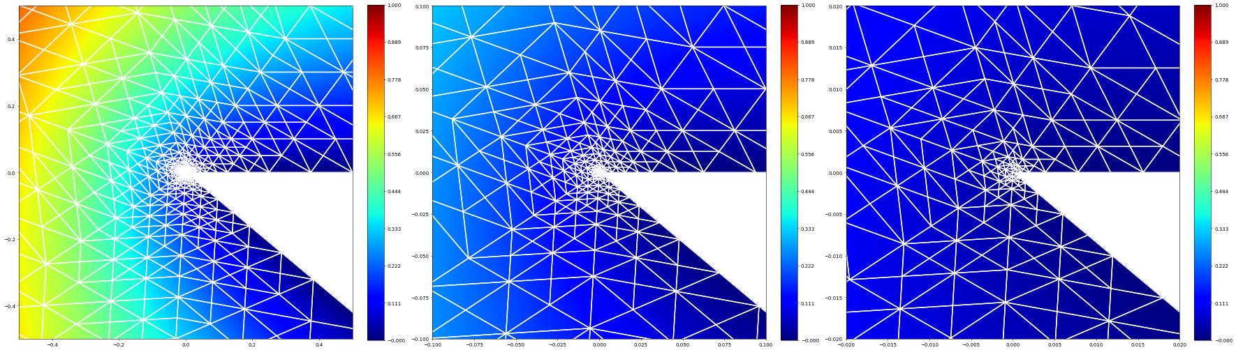
Let’s have a look at the center of the domain:

pyplot.close('all')
fig = pyplot.figure(figsize=(35,15))
plot(uh, figure=(fig, 131), xlim=(-0.5, 0.5), ylim=(-0.5, 0.5),
        gridLines="white", colorbar={"shrink": 0.75}, linewidth=2)
plot(uh, figure=(fig, 132), xlim=(-0.1, 0.1), ylim=(-0.1, 0.1),
        gridLines="white", colorbar={"shrink": 0.75}, linewidth=2)
plot(uh, figure=(fig, 133), xlim=(-0.02, 0.02), ylim=(-0.02, 0.02),
        gridLines="white", colorbar={"shrink": 0.75}, linewidth=2)

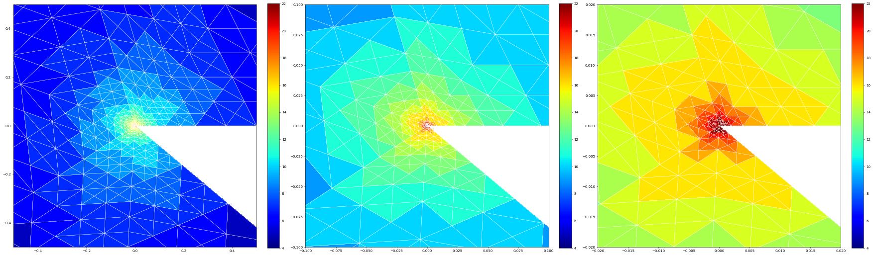
We can also visualize the grid levels used

fig = pyplot.figure(figsize=(35,15))
from dune.fem.function import levelFunction
levels = levelFunction(uh.space.gridView)
plot(levels, figure=(fig, 131), xlim=(-0.5, 0.5), ylim=(-0.5, 0.5),
        gridLines="white", colorbar={"shrink": 0.75}, linewidth=0.5)
plot(levels, figure=(fig, 132), xlim=(-0.1, 0.1), ylim=(-0.1, 0.1),
        gridLines="white", colorbar={"shrink": 0.75}, linewidth=0.5)
plot(levels, figure=(fig, 133), xlim=(-0.02, 0.02), ylim=(-0.02, 0.02),
        gridLines="white", colorbar={"shrink": 0.75}, linewidth=0.5)

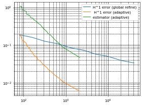
Finally, let us compare the globally refined solution and the adaptive one plotting number of degrees of freedom versus the error and the estimator

pyplot.close('all')
pyplot.loglog(dofsGlobal,errorGlobal,label="H^1 error (global refine)")
pyplot.loglog(dofs,errorVector,label=" H^1 error (adaptive)")
pyplot.loglog(dofs,estimateVector,label="estimator (adaptive)")
pyplot.grid(visible=True, which='major', color='black', linestyle='-')
pyplot.grid(visible=True, which='minor', color='black', linestyle='--')
pyplot.legend(frameon=True,facecolor="white",framealpha=1)

<matplotlib.legend.Legend at 0x7f3378cabb20>

This page was generated from the notebook laplace-adaptive_nb.ipynb and is part of the tutorial for the dune-fem python bindings