Section author: Andreas Dedner <a.s.dedner@warwick.ac.uk>, Robert Klöfkorn <robert.kloefkorn@iris.no>, Martin Nolte <nolte.mrtn@gmail.com>
Adaptivity and Moving Domains: extended grid views
Overview and some basic grid views (level and filtered)
When constructing a grid, the object returned to Python is always the so called LeafGridView. Without any refinement this is simply a view on all the elements of the grid. As soon as the grid is refined the leaf grid view changes so that it always contains the leaf elements the grid, i.e., the elements on the finest level. Since it is a read only view refinement is carried out using the underlying hierarchical grid, i.e.,
grid.hierarchicalGrid.globalRefine(1)
For a given hierarchical grid one can use different views, i.e., a view on all the elements of a given level:
DUNE-FEM provides a number of additional views which will be discussed further in this chapter:
dune.fem.view.adaptiveLeafGridView: this view should be used when the grid is supposed to be locally adapted. The view is still on the leaf elements of the grid but way data is attached to the entities of the grid is optimized for frequent grid changes as caused by local adaptivity. Its usage is shown in the following examples.
dune.fem.view.geometryGridView: this is an example of a meta grid view which is constructed from an existing grid view and replaces some aspect - in this case the geometry of each element using a given grid function. This concept makes it easy to perform simulations for example on complex domains or on moving grids as shown in Evolving Domains.
dune.fem.view.filteredGridView: allows the user to select a subset of a given grid view by providing a filter on the elements. In its simplest version only the iterator is replaced with an iterator over the elements in the filter but in addition it is also possible to obtain a new index set with indices restricted to the elements in the filter.
Dynamic Local Grid Refinement and Coarsening
For refining and coarsening a grid locally the dune.fem module provides a function adapt. The storage of all discrete functions will be automatically resized to accommodate the changes in the grid but the resulting dof vector will not be initialized. To prolong and restrict data from the old to the new grid, the corresponding discrete functions have to be passed to the dune.fem.adapt method:
fem.adapt(u1,u2,...,uN)
The module dune.fem also provides a globalRefine(level,*dfs) method, where a negative level globally coarsens the grid. If discrete functions are passed in they will be prolonged (restricted) and resized correctly, the dof vectors of all other discrete functions will only be resized, i.e. stored data will be lost.
Note
All the prolongation/restriction described here requires that the discrete spaces were constructed over an adaptiveLeafGridView.
So the code has to be modified for example as follows
from dune.alugrid import aluConformGrid as leafGridView
from dune.fem.view import adaptiveLeafGridView as adaptiveGridView
gridView = adaptiveGridView( leafGridView(domain) )
Note
if the underlying storage of a discrete function is stored on the Python side as a numpy array, i.e., vec = uh.as_numpy was called, then access to vec will be undefined after a grid modification since the underlying buffer change will not have been registered.
The module dune.fem provides a function for marking elements for refinement/coarsening:
def mark(indicator, refineTolerance, coarsenTolerance=0,
    minLevel=0, maxLevel=None):
where indicator is a grid function.
An element \(T\) is marked for refinement if the value of indicator
on \(T\) is greater then refineTolerance and coarsened if the
value is less then coarsenTolerance. The element \(T\) is not
refined if its level is already at maxLevel and not coarsened if its
level it at minLevel. This method can for example be used to refine
the grid according to an equal distribution strategy by invoking
dune.fem.mark(indicator, theta/grid.size(0))
where theta is a given tolerance.
A layered Doerfler strategy is also available
def doerflerMark(indicator, theta, maxLevel=None, layered=0.05):
The following two examples showcase adaptivity: the first one using a residual a-posteriori estimator for an elliptic problem, the second one shows adaptivity for a time dependent phase field model for crystal growth. At the end of this section a dual weighted residual approach is used to optimize the grid with respect to the error at a given point. While the first two examples can be implemented completely using the available Python bindings the final example requires using a small C++ snippet which is easy to integrate into the Python code.
Evolving Domains
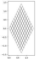
As mentioned above DUNE-FEM provides a grid view that makes it easy to exchange the geometry of each entity in the grid. To setup such a grid view one first needs to construct a standard grid view, i.e., a leafGridView and define a grid function over this view using for example a discrete function, a UFL function, or one of the concepts described in the section Grid Function. Note that the topology of the grid does not change, i.e., how entities are connected with each other. The following shows an example of how to change a grid of the unit square into a grid of a diamond shape:
from matplotlib import pyplot
from ufl import sqrt, SpatialCoordinate, as_vector
import dune.ufl
from dune.grid import structuredGrid
from dune.fem.view import geometryGridView
from dune.fem.function import gridFunction
square = structuredGrid([0,0],[1,1],[10,10])
x = SpatialCoordinate(dune.ufl.cell(2))
transform = as_vector([ (x[0]+x[1])/sqrt(2), (-x[0]+x[1])*sqrt(2) ])
diamond = gridFunction(transform,square,order=1,name="diamond")
diamond = geometryGridView(diamond)
diamond.plot()
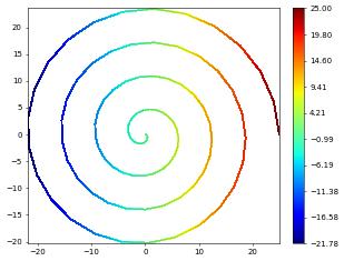
In a second example we embed a 1D interval into 3D:
from ufl import cos,sin
square = structuredGrid([0],[25],[100])
theta = SpatialCoordinate(dune.ufl.cell(1))[0]
transform = as_vector([cos(theta),sin(theta)])*(25-theta)
diamond = gridFunction(transform,square,order=1,name="diamond")
spiral = geometryGridView(diamond)
Note: currently plotting for 1d grids is not implemented spiral.plot() but we can plot some grid function, e.g., given by ufl expressions
from dune.fem.plotting import plotPointData as plot
plot(theta, gridView=spiral)
By using a discrete function to construct a geometry grid view, it becomes possible to simulate problems on evolving domains where the evolution is itself the solution of the partial differential equation. We demonstrate this approach based on the example of surface mean curvature flow first in its simplest setting and then with the evolution of the surface depending on values of a computed surface quantity satisfying a heat equation on the surface:
Todo
add a coupled surface diffusion/evolution problem