Alternative Solvers (Scipy and Petsc)

Here we look at different ways of solving PDEs using external packages. Different linear algebra backends can be accessed by changing setting the storage parameter during construction of the discrete space. All discrete functions and operators/schemes based on this space will then use this backend. Available backends are numpy,istl,petsc. The default is numpy which uses simple data structures and linear solvers implemented in the dune-fem package - these backends were discussed in the previously section.

As discussed there, a degrees of freedom vector (dof vector) can be retrieved from a discrete function over the numpy space by using the as_numpy method. Similar attributes are available for the other storages, i.e., as_istl,as_petsc. These attributes are also available to retrieve the underlying matrix structures of linear operators. We will show now how to use this to use scipy or petsc4py to solve the (non) linear systems.

We start with the same setup as used in the previously section:

import matplotlib.pyplot as plt
import numpy

from dune.grid import structuredGrid as leafGridView
from dune.fem.space import lagrange
from dune.fem import integrate
from ufl import TestFunction, TrialFunction, SpatialCoordinate, FacetNormal, \
                dx, ds, div, grad, dot, inner, exp, sin, conditional

gridView = leafGridView([0, 0], [1, 1], [24, 24])
space = lagrange(gridView, order=2)
u_h = space.interpolate(0, name='u_h')

x,u,v,n = ( SpatialCoordinate(space), TrialFunction(space), TestFunction(space), FacetNormal(space) )
exact = 1/2*(x[0]**2+x[1]**2) - 1/3*(x[0]**3 - x[1]**3) + 1

a  = ( inner(grad(u),grad(v)) + (1+u)**2*u*v ) * dx
bf = (-div(grad(exact)) + (1+exact)**2*exact) * v * dx
bg = dot(grad(exact),n)*v*ds

# simple function to show the result of a simulation
def printResult(method,error,info):
    print(method,"L^2, H^1 error:",'{:0.5e}, {:0.5e}'.format(
                 *[ numpy.sqrt(e) for e in integrate([error**2,inner(grad(error),grad(error))]) ]),
          "\n\t","solver info=",info,flush=True)

We will use the galerkin operator from dune.fem.operator instead of the scheme used so far, since we do not need the solve method since we want to use external solvers in this section:

from dune.fem.operator import galerkin
from dune.ufl import DirichletBC
operator = galerkin([a - (bf+bg), DirichletBC(space,exact,2)])

Accessing underlying data structures

The most important step is accessing the data structures setup on the C++ side in Python. In this case we would like to use the underlying dof vector from a discrete function as numpy arrays and system matrices assembled by the schemes and operators as scipy sparse matrices.

In the introduction we already discussed the as_numpy attribute which allows access to the degrees of freedom as numpy array based on the python buffer protocol. So no data is copied and changes to the dofs made on the Python side are automatically carried over to the C++ side.

We setup u_h to be zero but can initialize the dof vector with a random values directly changing u_h itself:

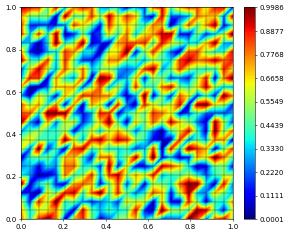
u_h.as_numpy[:] = numpy.random.rand(space.size)
u_h.plot()

Tip

changes to the numpy array u_h.as_numpy carries over to the discrete function u_h, just remember to make changes using vecu_h[:] to change the actual memory buffer.

An instance of dune.fem.operator describing an operator L provides a method linear which returns an object that stores a sparse matrix structure. The object describes the operator linearized around zero. To linearize around a different value use the jacobian method on the operator that linearized the the operator L around a given grid function ubar and fills the linear operator structure passed in as second argument. It is also possible to pass assemble=False to the linear method to avoid an the linearization around zero to reduce computational cost:

linOp = operator.linear()                  # linearized around 0
linOp = operator.linear(assemble=False)    # empty (non valid) linear operator
operator.jacobian(space.zero, linOp)       # linearized around zero

Here we linearize around zero. But that argument could be any grid function. A second version of this method will return an addition discrete function rhs which equals -L[ubar] such that DL[ubar](u-ubar) - rhs are the first terms in the Taylor expansion of the operator L:

rhs = u_h.copy()
operator.jacobian(u_h, linOp, rhs)

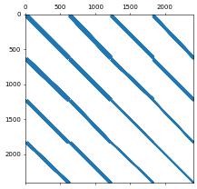
One can now easily access the underlying sparse matrix by again using as_numpy (and again the underlying data buffers are not copied):

A = linOp.as_numpy
print(type(A))
plt.spy(A, precision=1e-8, markersize=1)

<class 'scipy.sparse._csr.csr_matrix'>

<matplotlib.lines.Line2D at 0x7f687580da50>

Defining discrete function with given external dof vector

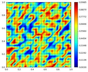
As a last step we sometimes need to construct a discrete function based on a given dof vector. Here a simple example where we use a numpy random vector as dof vector for a discrete function:

v_coeff = numpy.random.rand(space.size)
vh = space.function("random", dofVector=v_coeff)
vh.plot()

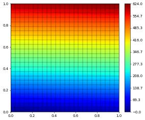
Again the dof vector is not copied so changing the numpy array will directly change the discrete function

v_coeff[:] = range(space.size)
vh.plot()

Now we have all the ingredients to write a simple Newton solver to solve our non-linear time dependent PDE.

Using Scipy

In our first example, we implement a simple Newton Krylov solver using a cg solver from Scipy.

Note

As pointed out the system matrix is no longer symmetric due to the handling of the Dirichlet constraints. For this reason we need to provide an initial guess to the cg solver with the degrees of freedom on the boundary set to be equal to the corresponding degrees of freedom in the right hand side vector. For this we use the setConstraints method on the solver.

import numpy as np
from scipy.sparse.linalg import cg
class Scheme1:
    def __init__(self, op):
        self.model = op.model
        self.jacobian = op.linear()
        self.op = op
        self.linIter = 0

    def callback(self,x):
        self.linIter += 1

    def solve(self, target):
        # create a copy of target for the residual
        res = target.copy(name="residual")
        initialGuess = target.copy(name="initial-guess")

        # extract numpy vectors from target and res
        sol_coeff = target.as_numpy
        res_coeff = res.as_numpy
        x0 = initialGuess.as_numpy

        n = 0
        while True:
            self.op(target, res)
            absF = numpy.sqrt( np.dot(res_coeff,res_coeff) )
            if absF < 1e-6:
                break
            self.op.jacobian(target,self.jacobian)
            self.op.setConstraints(res,initialGuess)
            dh_coeff = cg(self.jacobian.as_numpy, res_coeff, x0,
                          callback=lambda x: self.callback(x) )
            sol_coeff -= dh_coeff[0]
            n += 1
        return {"iterations":n, "linear_iterations":self.linIter}

scheme1_cls = Scheme1(operator)
u_h.interpolate(2)
info = scheme1_cls.solve(target=u_h)
printResult("Scipy-1",u_h-exact,info)
u_h.plot()

Scipy-1 L^2, H^1 error: 1.17613e-06, 1.83002e-04
         solver info= {'iterations': 4, 'linear_iterations': 799}

We can also use a non linear solver from the Scipy package - together for example with an incomplete LU factorization for the Jacobian.

Note

since we are using a LU type method here (i.e. a direct solver) we do not need to worry about the constraints as with the cg method previously.

from scipy.optimize import newton_krylov, root
from scipy.sparse.linalg import LinearOperator,spilu

class Scheme2:
    def __init__(self, op):
        self.op = operator
        self.model = op.model
        self.res = u_h.copy(name="residual")
        self.linIter = 0

    def callback(self,x):
        self.linIter += 1
    def cgCallback(self,*args,**kwargs):
        return cg(*args,**kwargs,callback=lambda x:self.callback(x))

    # non linear function
    def f(self, x_coeff):
        # the following converts a given numpy array
        # into a discrete function over the given space
        x = space.function("tmp", dofVector=x_coeff)
        self.op(x, self.res)
        return self.res.as_numpy

    # class for the derivative DS of S
    class Df(LinearOperator):
        def __init__(self, op, x_coeff):
            self.op = op
            self.shape = (x_coeff.shape[0], x_coeff.shape[0])
            self.dtype = x_coeff.dtype
            x = space.function("tmp", dofVector=x_coeff)
            self.jacobian = self.op.linear()
            self.n = -1
            self.update(x_coeff,None)
        # reassemble the matrix DF(u) given a DoF vector for u
        def update(self, x_coeff, f):
            x = space.function("tmp", dofVector=x_coeff)
            self.op.jacobian(x, self.jacobian)
            self.invJac = spilu(self.jacobian.as_numpy.tocsc())
            self.n += 1
        # compute DS(u)^{-1}x for a given DoF vector x
        def _matvec(self, x_coeff):
            return self.invJac.solve(x_coeff)


    def solve(self, target):
        sol_coeff = target.as_numpy
        M = self.Df(self.op,sol_coeff)
        # call the newton krylov solver from scipy
        sol_coeff[:] = newton_krylov(self.f, sol_coeff,
                    f_tol=1e-6, method=self.cgCallback, inner_M=M)
        return {"iterations":M.n, "linear_iterations":self.linIter}

scheme2_cls = Scheme2(operator)
u_h.interpolate(2)
info = scheme2_cls.solve(target=u_h)
printResult("Scipy-2",u_h-exact,info)
u_h.plot()

Scipy-2 L^2, H^1 error: 1.17613e-06, 1.83002e-04
         solver info= {'iterations': 4, 'linear_iterations': 16}

Using PETSc4Py

The following requires that a PETSc installation was found during the configuration of dune. Furthermore the Python package `petsc4py is required:

from dune.common.checkconfiguration import assertCMakeHave, ConfigurationError
try:
    assertCMakeHave("HAVE_PETSC")
    petsc = True
except ConfigurationError:
    print("Dune not configured with petsc - skipping example")
    petsc = False
try:
    import sys
    import petsc4py
    petsc4py.init(sys.argv)
    from petsc4py import PETSc
except ModuleNotFoundError:
    print("petsc4py module not found -- skipping example")
    petsc4py = None

To use petsc4py we need to which to a storage based on the PETSc package using the storage argument to the space constructor.

Implementing a Newton Krylov solver using the binding provided by petsc4py is now straightforward - we again use incomplete LU as preconditioner:

if petsc4py is not None and petsc:
    petsc_options = PETSc.Options()
    spacePetsc = lagrange(gridView, order=2, storage='petsc')
    u_h = spacePetsc.interpolate(2, name='u_h')  # start with solution at top boundary
    opPetsc = galerkin([a==bf+bg,DirichletBC(spacePetsc,exact,2)],
                       domainSpace=spacePetsc,rangeSpace=spacePetsc)

    class Scheme3:
        def __init__(self, op):
            self.op = op
            self.jacobian = op.linear()
            self.ksp = PETSc.KSP()
            self.ksp.create(PETSc.COMM_WORLD)
            # use conjugate gradients method
            self.ksp.setType("cg")
            # use sor preconditioner
            # self.ksp.getPC().setType("sor")
            # or ILU(1)
            self.ksp.getPC().setType("ilu")
            petsc_options['pc_factor_levels'] = 1
            self.ksp.setOperators(self.jacobian.as_petsc)
            self.ksp.setInitialGuessNonzero(True)
            self.ksp.setFromOptions()
        def solve(self, target):
            res = target.copy(name="residual")
            dh = target.copy(name="direction")
            sol_coeff = target.as_petsc
            dh_coeff = dh.as_petsc
            res_coeff = res.as_petsc
            n = 0
            numIter = 0
            while True:
                self.op(target, res)
                absF = numpy.sqrt( np.dot(res_coeff,res_coeff) )
                if absF < 1e-6:
                    break
                dh.clear()
                self.op.jacobian(target,self.jacobian)
                self.op.setConstraints(res,dh) # petsc does not seem to need this...
                self.ksp.setUp()
                self.ksp.solve(res_coeff, dh_coeff)
                numIter += self.ksp.getIterationNumber()
                sol_coeff -= dh_coeff
                n += 1
            return {"iterations":n, "linear_iterations":numIter}

    u_h.interpolate(2)
    scheme3_cls = Scheme3(opPetsc)
    info = scheme3_cls.solve(target=u_h)
    printResult("PETSc4py 1",u_h-exact,info)
    u_h.plot()

PETSc4py 1 L^2, H^1 error: 1.17613e-06, 1.83002e-04
         solver info= {'iterations': 4, 'linear_iterations': 52}

Here is another example now using the petsc4py bindings for the non linear KSP solvers from PETSc. This time we use a algebraic multigrid preconditioner:

if petsc4py is not None and petsc is not None:
    class Scheme4:
        def __init__(self, op):
            self.op = op
            self.res = op.rangeSpace.interpolate(0,name="residual")
            self.jacobian = op.linear()
            self.snes = PETSc.SNES().create()
            self.snes.setFunction(self.f, self.res.as_petsc.duplicate())
            self.snes.setUseMF(False)
            self.snes.setJacobian(self.Df, self.jacobian.as_petsc, self.jacobian.as_petsc)
            self.snes.setTolerances(atol=1e-6)
            self.snes.getKSP().setType("cg")
            self.snes.getKSP().getPC().setType("hypre")
            petsc_options['pc_hypre_type'] = 'boomeramg'
            self.snes.setFromOptions()

        def f(self, snes, x, f):
            # setup discrete function using the provide petsc vectors
            inDF = self.op.domainSpace.function("tmp",dofVector=x)
            outDF = self.op.rangeSpace.function("tmp",dofVector=f)
            self.op(inDF,outDF)

        def Df(self, snes, x, m, b):
            inDF = self.op.domainSpace.function("tmp",dofVector=x)
            self.op.jacobian(inDF, self.jacobian)
            return PETSc.Mat.Structure.SAME_NONZERO_PATTERN

        def solve(self, target):
            sol_coeff = target.as_petsc
            self.res.clear()
            self.snes.solve(self.res.as_petsc, sol_coeff)
            return {"iterations":self.snes.getIterationNumber(),
                    "linear_iterations":self.snes.getLinearSolveIterations()}

    scheme4_cls = Scheme4(opPetsc)
    u_h.interpolate(2)
    info = scheme4_cls.solve(target=u_h)
    printResult("PETSc4py 2",u_h-exact,info)
    u_h.plot()

PETSc4py 2 L^2, H^1 error: 1.17613e-06, 1.83002e-04
         solver info= {'iterations': 4, 'linear_iterations': 16}

This page was generated from the notebook solversExternal_nb.ipynb and is part of the tutorial for the dune-fem python bindings