Sampling the Solution over a Line

Let us revisit our simple 3d example from the introduction

from matplotlib import pyplot
import numpy
try:
    import pygmsh
    with pygmsh.geo.Geometry() as geom:
        poly = geom.add_polygon([
              [ 0.0,  0.5, 0.0], [-0.1,  0.1, 0.0], [-0.5,  0.0, 0.0],
              [-0.1, -0.1, 0.0], [ 0.0, -0.5, 0.0], [ 0.1, -0.1, 0.0],
              [ 0.5,  0.0, 0.0], [ 0.1,  0.1, 0.0] ], mesh_size=0.05)
        geom.twist(
            poly,
            translation_axis=[0, 0, 1], rotation_axis=[0, 0, 1], point_on_axis=[0, 0, 0],
            angle=numpy.pi / 3,
        )
        mesh = geom.generate_mesh(verbose=False)

    points, cells = mesh.points, mesh.cells_dict
    domain3d = {"vertices":points.astype("float"), "simplices":cells["tetra"]}
except ImportError: # pygmsh not installed - use a simple cartesian domain
    print("pygmsh module not found using a simple Cartesian domain - ignored")
    from dune.grid import cartesianDomain
    domain3d = cartesianDomain([-0.25,-0.25,0],[0.25,0.25,1],[30,30,60])

from dune.alugrid import aluSimplexGrid as leafGridView3d
gridView3d  = leafGridView3d(domain3d)

As before we solve a simple Laplace problem

from dune.fem.space import lagrange as solutionSpace
from dune.fem.scheme import galerkin as solutionScheme
from ufl import TrialFunction, TestFunction, SpatialCoordinate, dot, grad, dx, conditional, sqrt

space3d = solutionSpace(gridView3d, order=1)
u = TrialFunction(space3d)
v = TestFunction(space3d)
x = SpatialCoordinate(space3d)
scheme3d = solutionScheme((dot(grad(u),grad(v))+u*v)*dx ==
                        conditional(dot(x,x)<.01,100,0)*v*dx,
                        solver='cg')
uh3d = space3d.interpolate(0,name="solution")
info = scheme3d.solve(target=uh3d)

Instead of plotting this using paraview we want to only study the solution along a single line. This requires findings points \(x_i = x_0+\frac{i}{N}(x1-x0)\) for \(i=0,\dots,N\) within the unstructured grid. This would be expensive to compute on the Python so we implement this algorithm in C++ using the LineSegmentSampler class available in Dune-Fem. The resulting algorithm returns a pair of two lists with coordinates \(x_i\) and the values of the grid function at these points:

#include <vector>
#include <utility>
#include <dune/fem/misc/linesegmentsampler.hh>

template <class GF, class DT>
std::pair<std::vector<DT>, std::vector<typename GF::RangeType>>
sample(const GF &gf, DT &start, DT &end, int n)
{
  Dune::Fem::LineSegmentSampler<typename GF::GridPartType> sampler(gf.gridPart(),start,end);
  std::vector<DT> coords(n);
  std::vector<typename GF::RangeType> values(n);
  sampler(gf,values);
  sampler.samplePoints(coords);
  return std::make_pair(coords,values);
}

import dune.generator.algorithm as algorithm
from dune.common import FieldVector
x0, x1 = FieldVector([0,0,0]), FieldVector([0,0,1])
p,v = algorithm.run('sample', 'utility.hh', uh3d, x0, x1, 100)
x,y = numpy.zeros(len(p)), numpy.zeros(len(p))
length = (x1-x0).two_norm
for i in range(len(x)):
    x[i] = (p[i]-x0).two_norm / length
    y[i] = v[i][0]
pyplot.plot(x,y)

[<matplotlib.lines.Line2D at 0x7f85c93cc2b0>]

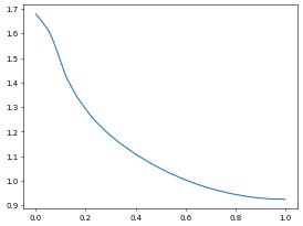
Note: the coordinates returned are always in the interval \([0,1]\) so if physical coordinates are required, they need to be rescaled. Also, function values returned by the sample function are always of a FieldVector type, so that even for a scalar example a v[i] is a vector of dimension one, so that y[i]=v[i][0] has to be used.

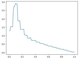
A mentioned above any grid function can be passed in as argument to the sample function. So for example plotting \(|\nabla u_h|\) is straight forward using the corresponding ufl expression. Since in this case automatic conversion from the ufl expression (available for example in the plotting function) to a grid function, we need to do this explicitly:

from dune.fem.function import gridFunction
absGrad = gridFunction(sqrt(dot(grad(uh3d),grad(uh3d))))
p,v = algorithm.run('sample', 'utility.hh', absGrad, x0, x1, 100)
for i in range(len(x)):
    y[i] = v[i][0]
pyplot.plot(x,y)

[<matplotlib.lines.Line2D at 0x7f85c9311370>]

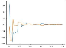
Similar we can plot both partial derivatives of the solution over the given line:

absGrad = gridFunction(grad(uh3d))
p,v = algorithm.run('sample', 'utility.hh', absGrad, x0, x1, 100)
dx,dy = numpy.zeros(len(p)), numpy.zeros(len(p))
for i in range(len(x)):
    dx[i] = v[i][0]
    dy[i] = v[i][1]
pyplot.plot(x,dx)
pyplot.plot(x,dy)

[<matplotlib.lines.Line2D at 0x7f85c81269d0>]

Remark: plotting over a line has been included as a utility function so can easily be called as shown below

from dune.fem.utility import lineSample
x,y = lineSample(uh3d,[0,0,0],[0,0,1],100)
pyplot.plot(x,y)

[<matplotlib.lines.Line2D at 0x7f85c932bbe0>]

The functions takes the two endpoints of the line and the number of (equidistant) sample points as arguments. By default the method throws an exception if part of the line is outside of the computational domain. This behavior can be disabled by setting the additional optional :code:bool parameter :code:allowOutside to :code:True.

Similar functions are available to obtain a :code:pointSample and to sample a grid function along the boundary (:code:boundarySample).

This page was generated from the notebook lineplot_nb.ipynb and is part of the tutorial for the dune-fem python bindings